6.5 - Hypotheses and critical regions
An unusual result might reflect a real change, or it might be ordinary random variation. You will turn a claim about a population into hypotheses, choose a rejection rule before observing the data, and explain what the resulting decision means. The rule controls how readily chance alone can lead you to reject a true claim.
Null and alternative hypotheses
A machine has historically produced a satisfactory item with probability . After an adjustment, of independently chosen items are satisfactory. Has the machine improved, or is this a lucky sample? The observed proportion describes these items; the question concerns the machine's underlying probability .
Null and alternative hypotheses
The null hypothesis, , specifies the population parameter used to calculate probabilities for the test. The alternative hypothesis, , describes the departure being investigated. For an improvement here, write and .
A test statistic is a quantity calculated from the observations and used to make the decision. Here, , the number of satisfactory items among , is convenient. Under , . The statistic is random before sampling; its observed value is .
The question you decide to investigate determines the tail:
| Departure investigated | Alternative | Results giving evidence against |
|---|---|---|
| An increase | Unusually large counts | |
| A decrease | Unusually small counts | |
| A change in either direction | Unusually small or large counts |
The first two are one-tailed tests; the third is two-tailed. Choose this direction from the investigation before looking at its result. Choosing whichever tail looks more striking after sampling changes the chance of rejection.
Worked example 1: investigating improvement
Question. An adjustment is intended to increase a machine's satisfactory-item probability from . State suitable hypotheses and a test statistic for independent items.
Plan. Define the population parameter, then translate “increase” into an inequality.
Let be the probability that an item produced after the adjustment is satisfactory. Then
Use . Under , ; large values support the alternative.
Answer. The hypotheses above define an upper-tailed test based on .
Check. The alternative describes improved production, whereas would describe only one observed sample.
Keep the population and sample size, but change the research question from improvement to any change. Now a deterioration matters too.
Worked example 2: investigating any change
Question. The machine's adjustment may change its satisfactory-item probability in either direction. State the hypotheses and identify the tail or tails.
Plan. Keep the null value but allow departures on both sides of it.
The same statistic is used, with under the null. Both unusually low and unusually high values can now give evidence of change.
Answer. A two-tailed test with the stated hypotheses.
Check. Both and satisfy the alternative; only the latter satisfies the previous example's alternative.
A hypothesis is about the population, so it should not say that the sample count or sample proportion equals its observed value.
Watch out
Write , not . The count need not equal its expected value even when the null hypothesis is true.
Translate a different investigation into a parameter statement.
Significance and rejection
A test needs a rule for deciding what counts as unusually far from the null model. Consider independent tosses of a coin and let be the number of heads. We investigate whether the coin favours heads, so and .
Under , a high count can still occur by chance. For example,
A rule that rejects for therefore rejects a fair coin on about of repeated samples of this size.
Critical region and significance level
The rejection region, or critical region, is the set of statistic values for which is rejected. The acceptance region is its complement: values for which is not rejected. A chosen significance level, such as , limits the probability of rejection when is true. For a discrete test, the actual probability may be smaller than this chosen level.
The regions concern possible results, not the unknown parameter. Here, is a rejection region and is its acceptance region. “Acceptance” is a conventional region name; it does not mean the null has been proved.
[DIAGRAM: asset_name: A discrete rejection region; asset_slug: hypotheses-binomial-region; caption: Seven or eight heads form a rejection region with null probability 9 over 256; description: A bar chart of B eight comma one half shows counts zero through eight. Counts seven and eight are shaded clay and labelled rejection region. Counts zero through six are pale blue and labelled acceptance region. The total null probability of the rejection region is 0.03515625, below the chosen five percent level.]
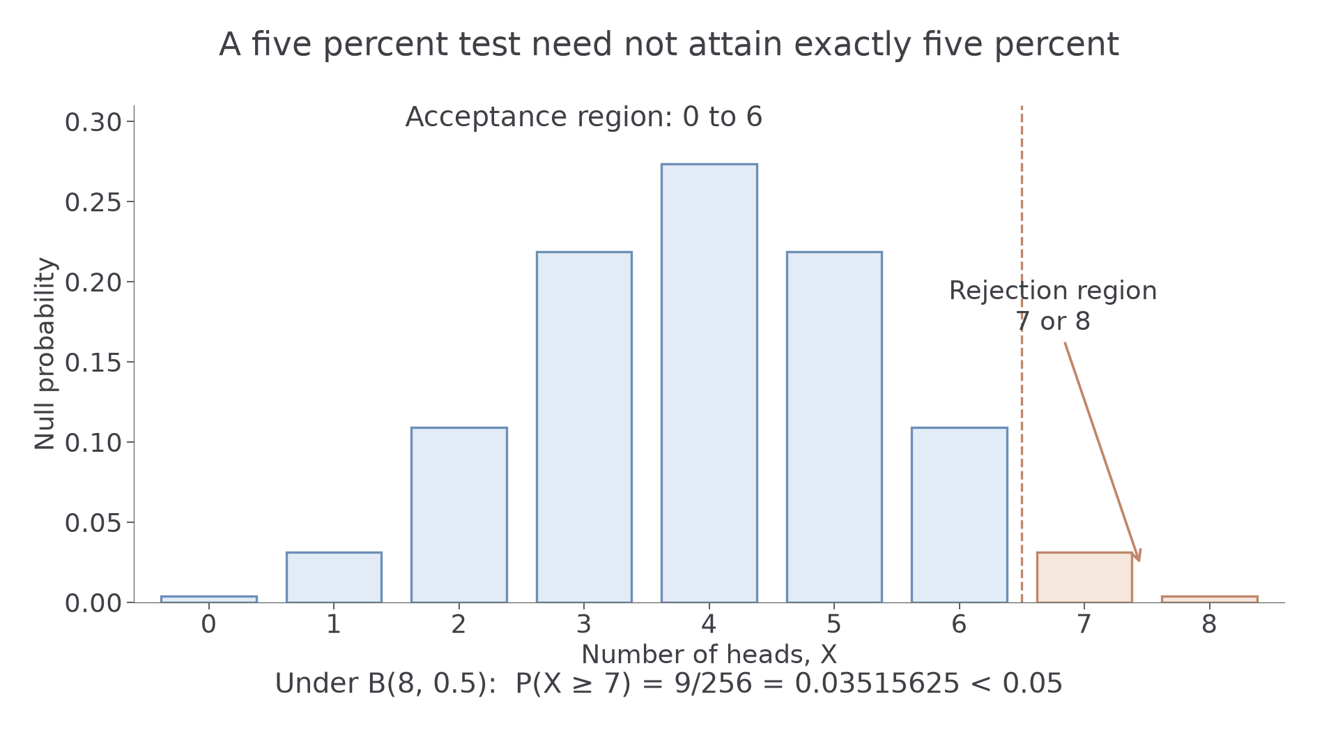
For a one-tailed test, choose the largest suitable tail region whose null probability does not exceed the level. A larger region would reject more often than allowed. For a two-tailed test at level , the usual equal-tail rule allocates to each tail. With discrete counts the attained tails need not have exactly equal probabilities, and their total may be below .
Continue this lesson.
You’re previewing NovaLearn without an account. Create a free account to read the rest.
Create free account