6.3 - Probability density functions
A continuous measurement can have zero probability at every single exact value and still have total probability one. In this first part of 6.3, you will explain that apparent puzzle using area, find probabilities from a density function, and handle distributions whose possible values extend indefinitely.
Density is not point probability
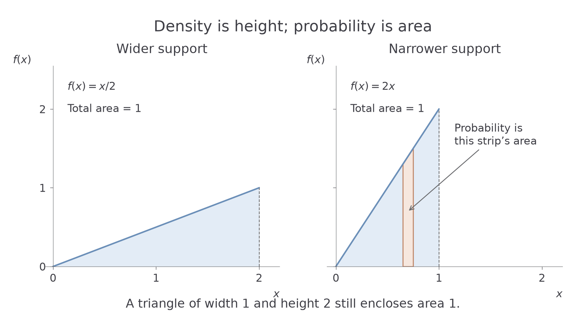
Can a probability density have height ? Yes: a height is not an area. A triangle of width and height has area , so it can represent a complete probability distribution.
A continuous random variable models measurements across an interval, rather than a list of separate scores. Its probability density function, written , tells us how probability is spread along that interval. Probability belongs to an area under the curve.
Probability density function
A probability density function is non-negative and has total area :
The interval where the density applies is its support; take elsewhere. Density may exceed , although an area's probability cannot.
For a continuous density, a single point has width zero and hence probability zero: . Thus including or excluding an endpoint does not change an interval probability. This is about an exact mathematical measurement. A reading rounded to may represent a whole interval of actual measurements, and that interval can have positive probability.
[DIAGRAM: asset_name: Density height and probability area; asset_slug: density-height-area; caption: A height of two is compatible with a total probability of one; description: Two triangular density graphs on matching horizontal and vertical scales. The left is f(x) equals x over two from zero to two, with height one and total area one. The right is f(x) equals two x from zero to one, with height two and total area one. A narrow highlighted strip on the right is labelled probability is area, not height.]
Worked example 1: normalising a triangle
Question. for , and otherwise. Find .
Plan. Make the triangle's total area equal to , then check non-negativity.
Its base is and height is , so
Answer. , giving on the support.
Check. Integration gives , and throughout the stated interval.
Change only the upper endpoint from to . The triangle must become taller to preserve its area.
Worked example 2: a density greater than one
Question. for , and otherwise. Find and for this density.
Plan. Normalise over the narrower support, then use the zero area of a point.
Although , a single point has no area.
Answer. and .
Check. The triangle has base and height , so its area is . Also : zero probability at the endpoint does not remove the probability accumulated before it.
Geometry can simplify normalisation for curved graphs too. A quarter-circle density of radius in the first quadrant has area , so total area one gives . You need not integrate a curve when its area is already known geometrically.
Watch out
Setting confuses height with area. Also check non-negativity: a function with integral but negative values on part of its interval is not a density.
Try a new interval, keeping both density conditions in mind.
Finding probabilities
For the density on , the probability between and is the area under that part of the line. It is not the difference in heights .
Probability as an integral
If ,
Use outside its support, or integrate only over the overlap of the event and the support. Endpoint inclusion makes no difference for a continuous density.
Not stated separately in the formula booklet: learn the area interpretation.
First sketch the support and mark the event. If the event extends beyond the possible values, trim its limits to the support. If it has no overlap, its probability is zero. Integrate a non-negative density in increasing order of limits so the resulting probability is non-negative.
Worked example 3: an event inside the support
Question. has density for , and zero otherwise. Find .
Plan. Integrate between the two event boundaries, both of which lie in the support.
Answer. .
Check. The region is a trapezium of width , with heights and . Its area is .
Keep the lower boundary and move only the upper boundary beyond the support. The probability stops accumulating at .
Continue this lesson.
You’re previewing NovaLearn without an account. Create a free account to read the rest.
Create free account