2.2, 3.2 - Straightening curved relationships
A curve can become a straight line when its axes use logarithms. In this shared part of 2.2 and 3.2, you will transform power and exponential relationships, connect gradients and intercepts to their constants, and recover the original model from a transformed graph. The axis labels will decide what each constant means.
Power laws
Could the same straight line describe two different curved relationships? Yes: it depends on what the axes measure. First consider a power law, such as , for positive . Taking logarithms brings the power down as a coefficient:
This is not linear in , but it is linear in the new coordinates , .
Linear form of a power law
For , with and ,
A graph of against has gradient and vertical intercept . The same form works with a single other logarithm base throughout. Not in the formula booklet: learn it.
“ against ” places horizontally and vertically. A vertical intercept occurs when , which means original input , not .
Worked example 1: a positive power
Question. Transform , , to linear form and state the gradient and vertical intercept of the transformed graph.
Plan. Take natural logarithms and compare with .
Answer. Plot against ; gradient , vertical intercept .
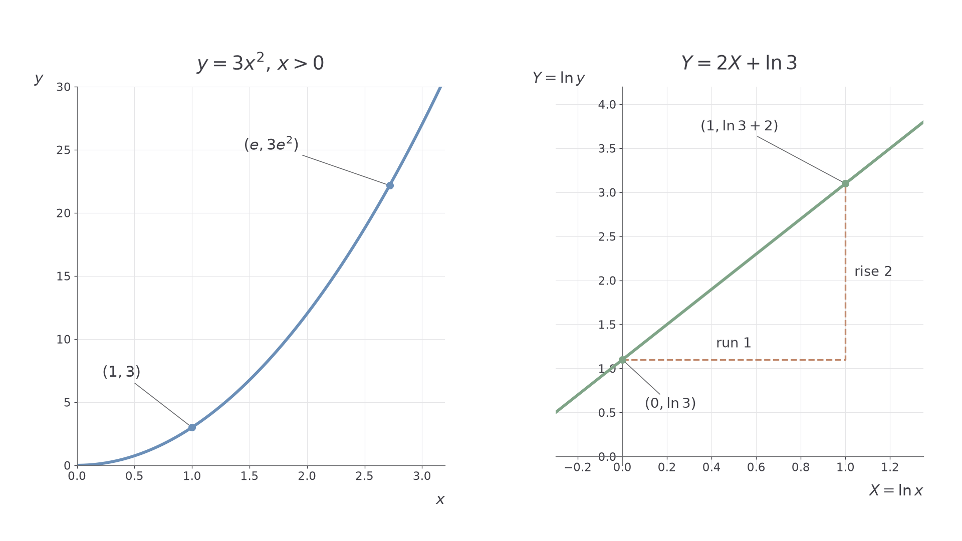
Check. At , , giving transformed point . At , , giving : a rise of for a run of .
Change only the sign of the power. The vertical intercept stays fixed, while the gradient reverses.
Worked example 2: a negative power
Question. Transform , , and state the same graph features.
Plan. Apply the power law to the negative exponent.
Answer. With the same log axes, gradient , vertical intercept .
Check. The transformed points at are and ; the rise is now . Both original outputs remain positive.
The curved positive-power relationship becomes an ordinary line when both coordinates are logged.
[DIAGRAM: asset_name: A power curve becomes a line; asset_slug: power-law-linearisation; caption: Logging both positive coordinates turns a power into the gradient; description: A left panel shows y equals 3x squared for positive x with points at x equals 1 and e. A right panel shows the corresponding straight line with horizontal coordinate X equals ln x and vertical coordinate Y equals ln y. Its marked points are 0 comma ln 3 and 1 comma ln 3 plus 2, with gradient 2 and vertical intercept ln 3.]
Watch out
The transformed intercept is , not . Recover by exponentiating. Also, a log-coordinate zero means original coordinate .
Transform a fractional power without changing its value.
Exponential relationships
In an exponential relationship the unknown input is an exponent, rather than the base being raised to a fixed power. For , taking logarithms gives . This is linear in and : the horizontal input itself stays unlogged.
Linear form of an exponential relationship
For , with , ,
A graph of against has gradient and vertical intercept . Equivalently, gives . Not in the formula booklet: learn it.
An exponential growth factor gives a positive transformed gradient. A decay factor gives a negative one. For , the original output is constant and the transformed line is horizontal.
Worked example 3: an exponential growth factor
Question. Transform to linear form and state suitable axes, gradient and vertical intercept.
Plan. Take natural logarithms and use .
Answer. Horizontal axis , vertical axis ; gradient , vertical intercept .
Check. At , . At , . The transformed rise is for a run of .
Replace the growth factor by its reciprocal. The transformed slope changes sign, with the same intercept.
Worked example 4: an exponential decay factor
Question. Transform and state the same features.
Plan. Use after taking logarithms.
Answer. Horizontal axis , vertical axis ; gradient , vertical intercept .
Check. At , , and its logarithm is , exactly the height given by the line.
For an exponential model, the transformed intercept occurs at original input , where . For a power model on two log axes it occurs at original input . Reading the horizontal label distinguishes them.
Continue this lesson.
You’re previewing NovaLearn without an account. Create a free account to read the rest.
Create free account