1.2 - Reversing a function
An inverse function recovers an input from its output, so the original function must be one–one. In this part of 1.2, you will rearrange rules to find inverses, use domain restrictions to choose the correct branch, and reflect graphs in the line .
Finding an inverse
A machine multiplies a number by , then subtracts . Its output is . How do you recover the input? Add , then divide by : . Reversing the calculation reverses both the operations and their order.
Inverse function
For a one–one function , the inverse function maps each output of back to its unique original input. The domain of is the range of , and the range of is the domain of .
The notation means the inverse function's output, not the reciprocal .
If a function is many–one, an output does not identify a unique input. It must first be restricted to a one–one domain before an inverse function can be defined.
To find a rule, write , solve for the original input in terms of the output , then rename the input of the inverse as . State the new domain using the original range.
Worked example 1: undoing a linear function
Question. Find the inverse of , .
Plan. Solve for , then exchange input and output roles.
The original linear function is one–one and has range .
Answer. , with domain and range .
Check. . In the other order, .
Change only the original domain. The inverse's algebraic expression stays the same, but its legal inputs and possible outputs change.
Worked example 2: swapping domain and range
Question. Find the inverse of , , stating its domain and range.
Plan. Find the original range, then use the rearranged linear rule.
Since the rule increases with ,
The same rearrangement as before gives the original input as .
Answer. , with domain and range .
Check. , so the included endpoint is preserved. Input to the inverse would return , excluded from the original domain, so is excluded from the inverse domain.
The two composition checks express the meaning of an inverse, but each has its own permitted inputs.
Inverse identities
For a one–one function ,
Not in the formula booklet: learn it.
A correct inverse rule cannot be used outside its domain just because its formula still produces a number.
Watch out
If , the reciprocal is , while the inverse is . Check an inverse by composition: it must undo the original function.
Now reverse a decreasing linear rule with a restricted domain.
Choosing the inverse branch
Rearranging a square introduces two algebraic candidates. The original domain decides which one can return an allowed original input. An inverse function must return one value, so leaving a sign is not a finished answer.
Recall that denotes the non-negative square root. From , the two possible signs describe the two sides of the vertex. The following pair changes only the domain to show how that sign is selected.
Worked example 3: the right-hand branch
Question. Find the inverse of , , stating its domain.
Plan. Rearrange the square and use to choose its sign.
The original minimum is attained at , so its range is .
Answer. , for .
Check. and . The inverse always returns a number at least , as required.
On the other branch, the square root is still non-negative. It is the expression before the root that must take the negative sign.
Worked example 4: the left-hand branch
Question. Find the inverse of , , stating its domain.
Plan. Use the original condition after rearranging.
The original range is again , since the vertex is included.
Answer. , for .
Check. , and . Choosing the plus sign would return , outside the original domain.
An odd power behaves differently. The real cube root is the unique real number whose cube is ; for example, . Cubing is one–one on all real numbers, so undoing a cube does not introduce a choice. Restrictions still determine the inverse domain.
Worked example 5: undoing a restricted cube
Question. Find the inverse of , , stating its domain.
Plan. Take the real cube root, and find the range from the negative value of .
For , , so and . Every output below occurs.
Answer. , for .
Check. , and . Input would return the excluded endpoint .
For a reciprocal square, first isolate the square. A strict restriction on one side of a vertical asymptote selects the sign, while the reciprocal also excludes a limiting output.
Worked example 6: a reciprocal square
Question. Find the inverse of , , stating its domain.
Plan. Isolate , then choose the negative root because .
The original range is : the reciprocal square is positive, can be arbitrarily small or large, and is never zero.
Answer. , for .
Check. , and . More generally, if , the inverse returns a number below , and substituting it into gives .
The input restrictions and the algebraic sign must agree throughout the inverse's domain.
Watch out
The domain in the reciprocal example describes original inputs. It selects the minus sign in the inverse rule. It is not the inverse domain: that comes from the original range .
Use the same reasoning with a shifted asymptote and a larger numerator.
Reflection in y equals x
If maps to , its inverse maps to . Therefore every point on the original graph becomes on the inverse graph. Swapping coordinates is a reflection in the line , drawn with equal scales on the axes.
Graph of an inverse
For a one–one function, reflect its graph in the mirror line to obtain the graph of its inverse. Included and excluded endpoints retain their inclusion status as their coordinates swap.
An -intercept becomes the inverse's -intercept . A -intercept becomes the inverse's -intercept . Only intercepts lying on the permitted original graph are available.
Worked example 7: reflecting a straight line
Question. Describe a sketch of , , and its inverse, identifying both graphs' intercepts and their mirror line.
Plan. Find the original intercepts, swap their coordinates, and use the inverse rule to check them.
The original graph passes through and . Reflection gives and .
Rearranging gives .
Answer. Draw the original line with gradient , its inverse with gradient , and the mirror line . Original intercepts are ; inverse intercepts are .
Check. The inverse rule gives and , confirming the reflected intercepts.
The mirror line belongs in an inverse sketch even when the two function graphs are easy to recognise.
[DIAGRAM: asset_name: Swapping coordinates; asset_slug: inverse-line-reflection; caption: Reflecting in y equals x swaps each point's input and output; description: Equal-scale coordinate axes show y equals 2x plus 1 in blue, y equals x minus 1 divided by 2 in green, and dashed mirror line y equals x. The point 0 comma 1 reflects to 1 comma 0 and the point 1 comma 3 reflects to 3 comma 1. Corresponding points are joined by faint perpendicular segments.]
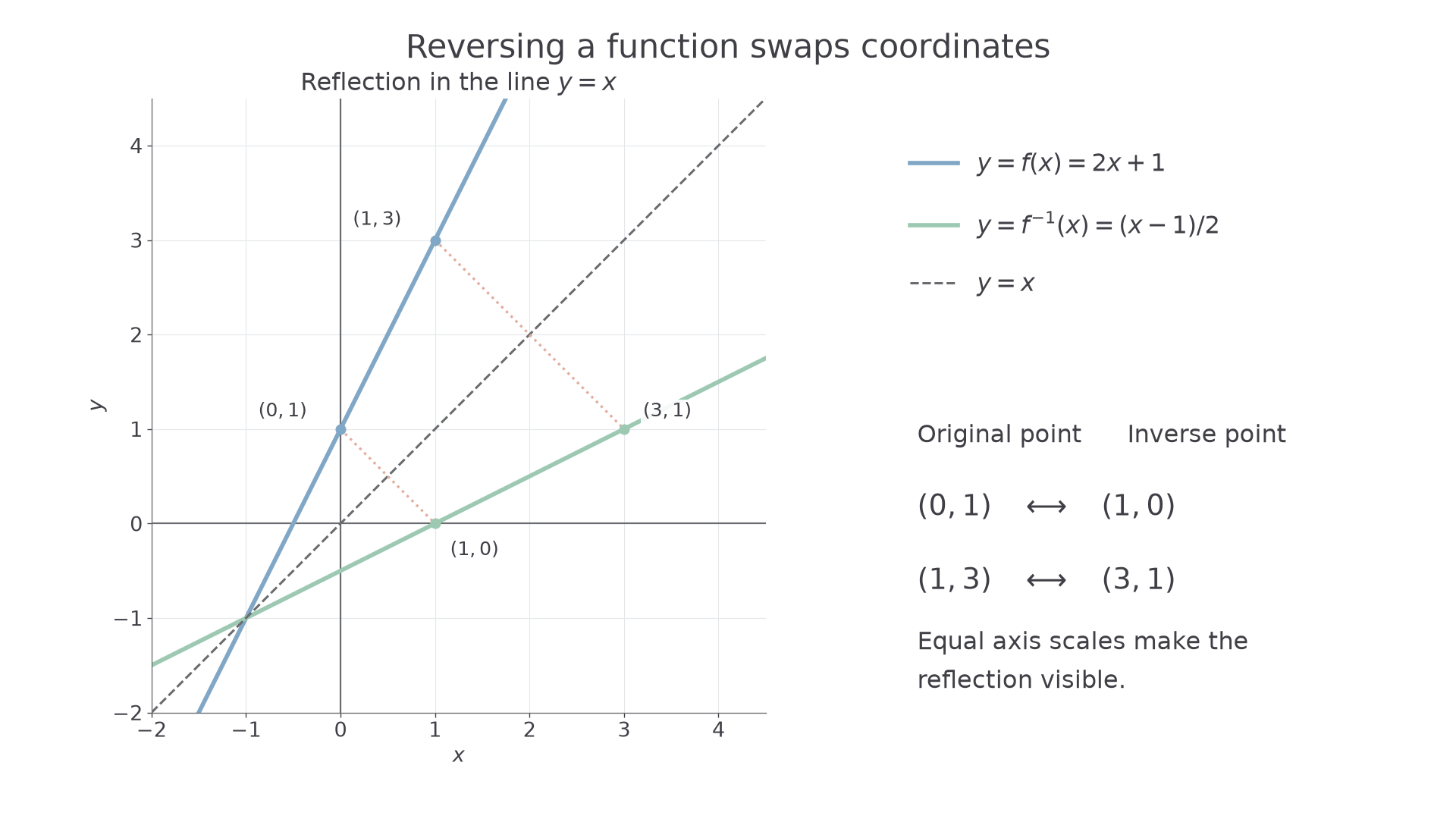
An asymptote describes a curve's limiting behaviour. At a vertical asymptote, the output grows in magnitude without bound as the input approaches a fixed value. A horizontal asymptote gives a height approached as the input increases or decreases without bound. Reflection swaps horizontal and vertical asymptotes: becomes , and becomes .
Replace the straight line by a reciprocal-square curve. The coordinate swap is unchanged, but now it also explains the positions of the asymptotes.
Worked example 8: reflecting asymptotes
Question. For , , describe the graph of its inverse, including its domain, range, asymptotes and the reflection of .
Plan. Swap the original domain and range, then reflect each feature in .
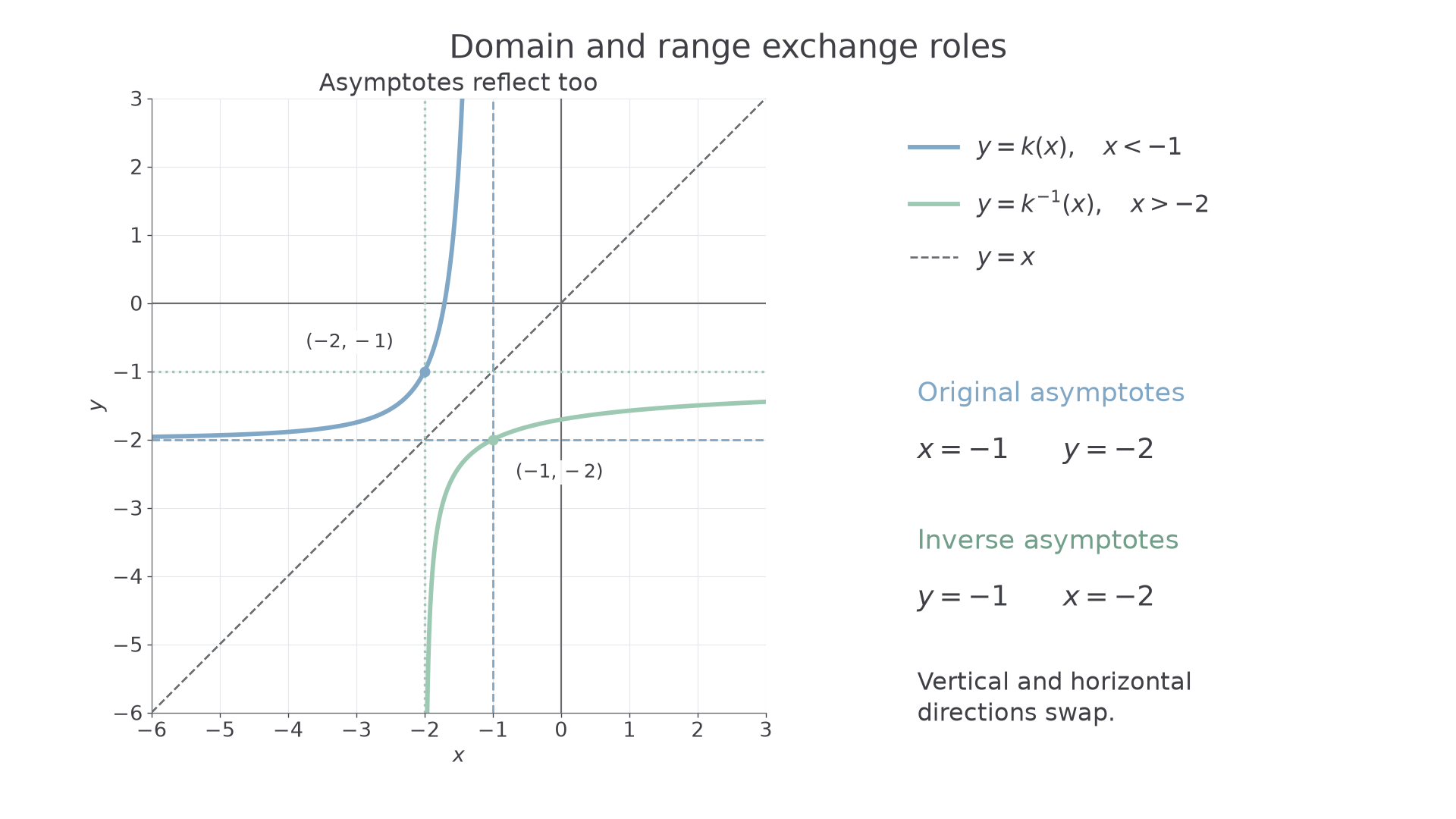
The original curve has vertical asymptote , horizontal asymptote , domain and range .
Answer. The inverse has domain , range , vertical asymptote and horizontal asymptote . The point becomes . Draw the reflected branch and the mirror line .
Check. Its rule gives . As approaches from above, the denominator approaches zero and the output decreases without bound; as increases, the output approaches from below.
The reflected graph lies to the right of its vertical asymptote and below its horizontal one, exactly as its domain and range require.
[DIAGRAM: asset_name: Asymptotes exchange direction; asset_slug: inverse-asymptote-reflection; caption: A vertical asymptote becomes horizontal when a function is reversed; description: Equal-scale axes show the branch y equals one divided by the square of x plus 1 minus 2 for x less than minus 1, and its reflected inverse y equals minus 1 minus one divided by the square root of x plus 2 for x greater than minus 2. Original asymptotes x equals minus 1 and y equals minus 2 are blue dashed lines; inverse asymptotes x equals minus 2 and y equals minus 1 are green dashed lines. The mirror line y equals x and the reflected pair minus 2 comma minus 1 and minus 1 comma minus 2 are labelled.]
Return to the machine in the opening: its input and output exchange places. The algebraic reversal and the graph's reflection express the same idea.
Exam tip
An inverse sketch should show the correct branch, its key features and the mirror line . Reflect the stated function's domain as well as its visible shape.
Reflect a set of features without needing a formula.
Quick Recap
- An inverse exists for a one–one function, and exchanges its domain and range.
- Rearrange to recover the original input, then rename variables and state the inverse domain.
- A square-root sign follows the original branch; a real cube root has no choice.
- Reflect points, endpoints and asymptotes in the line .
The opening machine is reversed by adding , then dividing by : returns to .