5.1 - Cumulative frequency and quartiles
A grouped table can tell you how many observations lie below a boundary even when the individual values are unknown. In this part of 5.1, you will build cumulative frequency graphs, find medians and quartiles, and compare datasets using box-and-whisker plots. You will distinguish exact summaries of raw data from estimates made within grouped classes.
Cumulative frequency
If people record their waiting times, how can you estimate the fraction who wait between and minutes without knowing each time? A running total turns that question into the difference between two graph readings.
Suppose waits are below minutes and a further are between and . Then waits are below , not .
Cumulative frequency
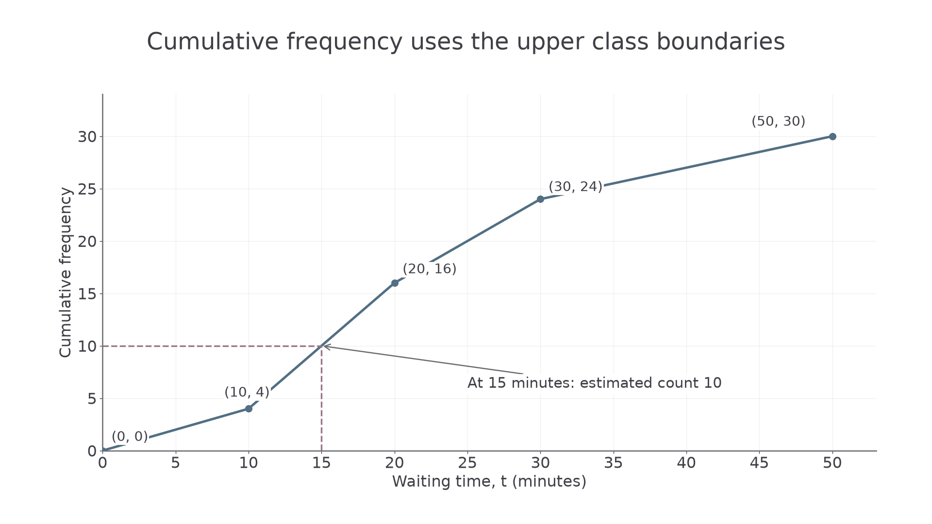
The cumulative frequency at a boundary is the total number of observations below that boundary. For grouped continuous data, add frequencies successively and plot the running totals against the upper class boundaries. Start with frequency zero at the lowest boundary.
Label both axes and use linear numerical scales. The graph cannot decrease: increasing the boundary cannot remove observations already counted. Join plotted points with an increasing curve when requested. Joining them with straight line segments gives the linear interpolation model used in this lesson: it assumes values are spread evenly within each class.
Worked example 1: plotting running totals
Question. Construct a cumulative frequency graph for these waiting times.
| Waiting time , minutes | Frequency | Cumulative frequency |
|---|---|---|
Plan. Add down the frequencies, then pair each running total with its upper boundary.
Plot
The first point records that no waits are below the lowest boundary. For example, means waits are below minutes.
Answer. The increasing graph below, joining the plotted points. It finishes at the total frequency .
Check. Differences between successive cumulative frequencies are , recovering the original frequencies. Plotting at the midpoints would attach those counts to the wrong waiting times.
The dashed reading at minutes will help answer the opening question.
[DIAGRAM: asset_name: Boundaries and running totals; asset_slug: data-cumulative-boundaries; caption: Plot cumulative frequencies at upper boundaries and begin at zero at the lowest boundary; description: Increasing piecewise linear cumulative frequency graph of waiting time with labelled points 0 comma 0, 10 comma 4, 20 comma 16, 30 comma 24, 50 comma 30. Dashed lines read across and down from the point 15 comma 10 to show an estimated count of 10 below 15 minutes. Both axes use numbered linear scales.]
Now keep the same running-total method but change how the measurements are recorded. Whole-number class labels for rounded measurements need continuous boundaries.
Worked example 2: measurements recorded to the nearest unit
Question. Lengths recorded to the nearest centimetre are grouped as follows. State the points for a cumulative frequency graph.
| Recorded length, cm | – | – | – |
|---|---|---|---|
| Frequency |
Plan. Convert the rounded classes to continuous boundaries, then use upper boundaries and running totals.
A recorded cm represents lengths up to cm; a recorded cm starts at cm. Thus the boundaries are , with successive totals .
Answer. Plot , , and , with length in cm horizontally and cumulative frequency vertically.
Check. Every class has width cm. The final total equals , and the first increase recovers the first frequency .
If a table instead says , those are already its boundaries; do not subtract . Nor should you introduce half-unit boundaries for an exact discrete count unless a continuous grouped model is actually being used.
To read a count below a given value, go vertically from the value to the graph, then horizontally to the cumulative-frequency axis. In Example 1, linear interpolation gives
Here denotes the estimated count below , rather than a proportion. Hence the estimated fraction between and minutes is . Above minutes, subtract from the total: waits. Boundary inclusion does not change these continuous-model estimates; exact discrete counts require their stated inequalities.
Watch out
The count between two values is the difference of two cumulative frequencies, not their sum. Divide by the total only when a proportion is requested.
Convert the next rounded table before choosing the plotting positions.
Medians, quartiles and percentiles
A percentile answers the reverse question: what value has a specified percentage of the observations below it? Instead of starting on the horizontal axis, start with a cumulative count.
Median, quartiles and percentiles
The median, , divides an ordered distribution into two halves. The lower quartile, , and upper quartile, , mark the lower and upper quarters. The interquartile range is , measuring the spread of the middle half. The percentile has approximately of observations below it.
For raw data, sort first. The median is the middle observation if the count is odd, or the mean of the two middle observations if it is even. To find raw-data quartiles here, take the median of the lower half and of the upper half; exclude the overall middle observation when the count is odd. For example, in , the median is , while the halves give and . Follow a convention explicitly stated in a question if one is supplied.
Worked example 3: exact quartiles from raw values
Question. Find the median and interquartile range of
Plan. Locate the middle pair of the full list, then the middle pair of each six-value half.
Answer. Median ; interquartile range .
Check. Six observations lie on either side of . The quartiles sit halfway between positions and , and between positions and , as required by the two halves.
The next example changes the information available: only grouped counts are known. Use cumulative levels , or for a percentile. Read across to the graph and down to the value axis. These are distribution estimates, not a rule telling you to round raw-data positions.
For straight-line interpolation within a class, the fraction of the class frequency needed is also the fraction of the class width needed.
Linear interpolation within a class
If a target cumulative count lies in a class with lower boundary , width , frequency , and cumulative frequency before that class,
This assumes an even spread within the class. Not in the formula booklet: learn the reasoning.
Continue this lesson.
You’re previewing NovaLearn without an account. Create a free account to read the rest.
Create free account