6.4 - The distribution of a sample mean
Individual measurements vary, and so do the means of repeated samples. In this part of 6.4, you will find the centre and spread of a sample mean, use its exact normal distribution for a normal population, and apply the Central Limit Theorem when a large sample makes normal approximation appropriate.
A mean as a random variable
If you multiply a sample size by four, does the sample mean become four times as precise? Its standard deviation halves. The square root in this relationship explains why obtaining a much more stable average can require many more observations.
Before a sample is taken, write its independent observations as , each from the same population with mean and variance . Their average
is itself a random variable. Different samples give different observed values, written .
The earlier linear-combination rules give
The independent variance contributions add before the total is divided by . No normal-population assumption was used for these two moment results.
Mean and variance of a sample mean
For independent observations from the same population, with finite mean and variance ,
The standard deviation of the sample mean is called its standard error.
The mean and variance appear in the formula booklet's sample-mean normal approximation. They also hold without normality; standard error is the square root of that variance.
The population standard deviation describes individual measurements. The standard error describes the means of samples of the specified size. Their units match, but they measure different variation.
Worked example 1: the spread of an average
Question. A population has mean and variance . For a random sample of independent observations, find the expectation, variance and standard error of its mean.
Plan. Keep the expectation at the population mean, divide variance by , then take a square root.
Answer. Expectation , variance , standard error .
Check. The individual standard deviation is . Dividing by gives , agreeing with the square root of the calculated variance.
Increase only the sample size, from to . Individual measurements retain the same spread.
Worked example 2: quadrupling the sample size
Question. For the same population, find the expectation, variance and standard error of a mean from independent observations.
Plan. Replace by in the sample-mean formulae.
Answer. Expectation , variance , standard error .
Check. The sample size is four times larger, its variance is one quarter as large, and its standard error is half as large. The population standard deviation is still .
For a sample without replacement from a large finite population, independence may be an approximation justified when the sample is a small fraction of that population. Use the supplied model. Recording one observation repeatedly does not produce independent information.
Watch out
The variance of a mean is , not . A sum of independent observations has variance ; averaging then divides that by .
Keep the population SD and standard error distinct in this check.
Normal populations
If the population is normal, its independent sample mean is exactly normal for every positive sample size. This follows from the earlier result that a linear combination of independent normal variables is normal. You do not need a large sample to establish normality in this case.
Sample mean from a normal population
If are independent, each with distribution , then
Standardise its value using
The sample-mean normal form is in the formula booklet under the CLT heading. Its exactness for a normal population and the standardisation step are not stated there separately: learn the distinction.
[DIAGRAM: asset_name: Individual measurements and sample means; asset_slug: sample-mean-spread; caption: Averaging leaves the centre fixed and reduces the standard deviation; description: Normal density curves for individual measurements N(100,64), means of sixteen with N(100,4), and means of sixty-four with N(100,1). All share centre one hundred. The three standard deviations are labelled eight, two and one. Each curve has total area one, and the narrowest curve is tallest.]
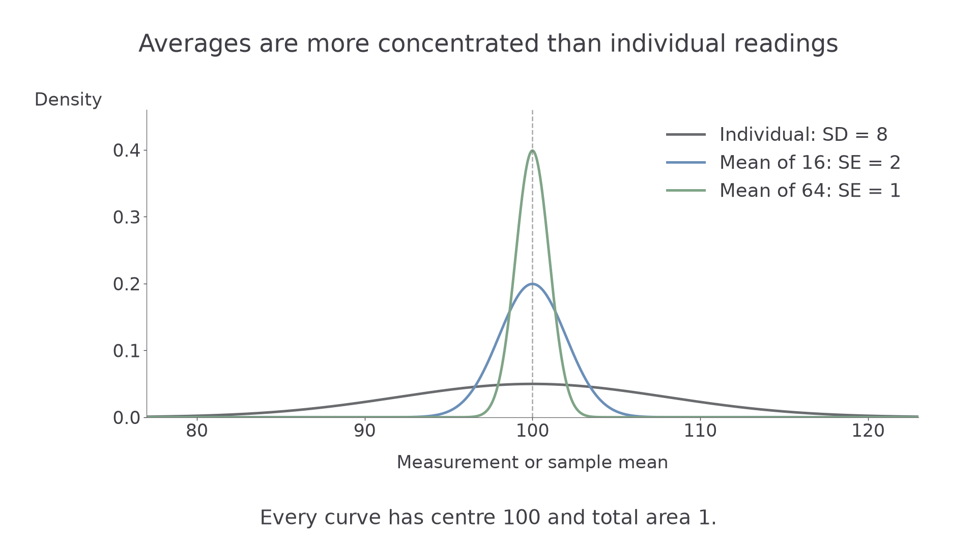
Use the normal tables just as before, but divide by the standard error of the mean. There is no continuity correction for the continuous measurements in the examples.
Worked example 3: an exact normal probability
Question. Individual measurements have distribution . A random sample of independent measurements is taken. Find the probability that its mean exceeds .
Plan. Identify the mean's normal distribution, then standardise with .
Answer. , to significant figures.
Check. A sample total has distribution . The event is total , giving , the same standardised boundary.
Continue this lesson.
You’re previewing NovaLearn without an account. Create a free account to read the rest.
Create free account