3.5 - Integration by substitution | Cambridge A-Level Mathematics

A change of variable can turn an unfamiliar integral into a familiar one. In this part of 3.5, you will use a supplied substitution to change every part of the integral, including its differential and, when appropriate, its limits. Algebraic and trigonometric examples will show why keeping the old and new variables separate matters.

Changing variables

What happens to $\int 2x\sqrt{x^2+1}\,\mathrm dx$ if we call $x^2+1$ by the shorter name $u$ ? The square root becomes $\sqrt u$ , and differentiation gives $\mathrm du/\mathrm dx=2x$ . Thus the whole combination $2x\,\mathrm dx$ becomes $\mathrm du$ . The new integral is simply $\int\sqrt u\,\mathrm du$ .

Integration by substitution

Integration by substitution changes the variable of an integral using a stated relationship. The relationship changes both the integrand and the differential, so the new integral contains only the new variable.

The method reverses the chain rule. If $u=g(x)$ , then differentiating $F(g(x))$ gives $F'(g(x))g'(x)$ . This explains why the differential factor is essential.

Changing the variable

If $u=g(x)$ , then $\mathrm du=g'(x)\,\mathrm dx$ , so

\int f(g(x))g'(x)\,\mathrm dx =\int f(u)\,\mathrm du.

For an indefinite result, substitute back to the original variable and include $C$ . This substitution rule is not listed separately in the formula booklet: reconstruct it from the chain rule.

The differential notation records the derivative relationship; it is not permission to change $x$ to $u$ without changing the rest of the integral. Use the given substitution, work out its derivative, then rewrite all remaining old-variable factors.

Worked example 1: a square-root power

Question. Use $u=x^2+1$ to find $\displaystyle\int2x\sqrt{x^2+1}\,\mathrm dx$ .

Plan. Replace $x^2+1$ by $u$ and the matching combination $2x\,\mathrm dx$ by $\mathrm du$ .

Since $u=x^2+1$ ,

\frac{\mathrm du}{\mathrm dx}=2x, \qquad \mathrm du=2x\,\mathrm dx.

Consequently

\begin{aligned} \int2x\sqrt{x^2+1}\,\mathrm dx &=\int u^{1/2}\,\mathrm du\\ &=\frac23u^{3/2}+C\\ &=\frac23(x^2+1)^{3/2}+C \end{aligned}

Answer. $\frac23(x^2+1)^{3/2}+C$ , valid for every real $x$ .

Check. Differentiation gives $(2/3)(3/2)(x^2+1)^{1/2}(2x)=2x\sqrt{x^2+1}$ . The inside expression is always positive.

Keep the substitution and change only the square root to its reciprocal. The differential conversion is unchanged; only the power of $u$ changes.

Worked example 2: a reciprocal square root

Question. Use $u=x^2+1$ to find $\displaystyle\int\frac{2x}{\sqrt{x^2+1}}\,\mathrm dx$ .

Plan. Use the same differential relationship, then integrate the new power $-1/2$ .

\begin{aligned} \int\frac{2x}{\sqrt{x^2+1}}\,\mathrm dx &=\int u^{-1/2}\,\mathrm du\\ &=2u^{1/2}+C\\ &=2\sqrt{x^2+1}+C \end{aligned}

Answer. $2\sqrt{x^2+1}+C$ , valid for every real $x$ .

Check. Its derivative is $2\times\frac12(x^2+1)^{-1/2}\times2x=2x/\sqrt{x^2+1}$ . At $x=0$ , both this derivative and the original integrand are zero.

We replaced the combination $2x\,\mathrm dx$ directly, so we did not need to divide by $x$ or invert $u=x^2+1$ . This avoids introducing an unnecessary restriction at $x=0$ . The derivative checks establish the displayed antiderivatives on their original domains.

Watch out

From $u=x^2+1$ , the line $\int2x\sqrt{x^2+1}\,\mathrm dx=\int2x\sqrt u\,\mathrm du$ is wrong: it retains the factor already absorbed by $\mathrm du=2x\,\mathrm dx$ . A transformed integral must have the correct differential factor and a single variable.

Use a new inner constant and power.

Transforming limits

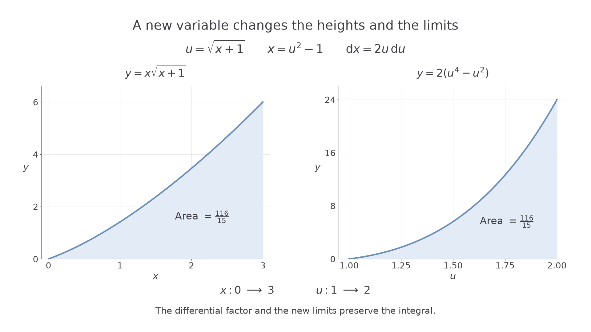
For a definite integral, the old limits describe values of $x$ . Convert them into values of the new variable before evaluating a transformed antiderivative. A small table keeps the correspondence visible.

The substitution may also require you to express $x$ itself in terms of $u$ . With $u=\sqrt{x+1}$ , we have $x=u^2-1$ and $\mathrm dx=2u\,\mathrm du$ . The root is the non-negative root, so $u\ge0$ ; this sign condition is part of the substitution.

Substitution with limits

For a valid change $u=g(x)$ on the interval,

\int_a^b f(g(x))g'(x)\,\mathrm dx =\int_{g(a)}^{g(b)}f(u)\,\mathrm du.

Use the transformed limits with a $u$ -antiderivative. Alternatively, return the antiderivative to $x$ and use the original limits. Do not mix these two routes.

The definite substitution rule is not listed separately in the formula booklet: it follows from the chain rule and definite integration.

Changing variables changes the integrand's height and the interval's width together. The two shaded regions below represent the same integral, although their graphs and horizontal scales differ.

[DIAGRAM: asset_name: The same integral in two variables; asset_slug: substitution-limits-area; caption: The substitution changes both the function and the limits while preserving the integral; description: The left coordinate plot shades y equals x times the square root of x plus one from x equals zero to three. The right shades y equals two times u to the fourth minus two times u squared from u equals one to two. Both areas are labelled 116 over 15. A linking label states u equals the square root of x plus one, x equals u squared minus one, and dx equals two u du.]
The substitution changes both the function and the limits while preserving the integral

Worked example 3: converting every old-variable factor

Question. Use $u=\sqrt{x+1}$ to find the exact value of $\displaystyle\int_0^3x\sqrt{x+1}\,\mathrm dx$ .

Plan. Express $x$ , the square root and $\mathrm dx$ in terms of $u$ , then convert both limits.

x=u^2-1,\quad \sqrt{x+1}=u,\quad \mathrm dx=2u\,\mathrm du.

The limits become

$x$	$0$	$3$
$u=\sqrt{x+1}$	$1$	$2$

Therefore

\begin{aligned} I&=\int_1^2(u^2-1)u(2u)\,\mathrm du\\ &=2\int_1^2(u^4-u^2)\,\mathrm du\\ &=2\left[\frac{u^5}{5}-\frac{u^3}{3}\right]_1^2\\ &=2\left(\frac{31}{5}-\frac73\right)=\frac{116}{15} \end{aligned}

Answer. $116/15$ .

Check. Rewriting $x=(x+1)-1$ directly gives the antiderivative $\frac25(x+1)^{5/2}-\frac23(x+1)^{3/2}$ . At $3$ and $0$ , its difference is also $116/15$ .

Continue this lesson.

You’re previewing NovaLearn without an account. Create a free account to read the rest.

Create free account

Last Accessed

Pure Mathematics 1

Advanced pure mathematics

Pure Mathematics 3 extensions

Pure Mathematics 2 only

Mechanics

Probability and Statistics 1

Probability and Statistics 2

3.5 - Integration by substitution

Changing variables

Transforming limits

Continue this lesson.

Learn faster with Nova