2.6, 3.6 - Locating a root
An equation can have a perfectly definite root without having a convenient exact expression for it. In 2.6 and 3.6, graphs will suggest where to look, and calculated signs will place a root inside a chosen interval. You will also show why a rounded answer is accurate and recognise when a sign change does not justify a conclusion.
Graphs suggest intervals
Where does ? Taking logarithms gives , which still has in two different forms. A graph can locate the solution even when algebra does not isolate it.
Plot and . At their intersection the two heights are equal, so its horizontal coordinate solves the equation. Alternatively, plot and look for its crossing of the -axis. These are two views of the same root.
Root and bracket
A root of is an input for which . A bracket is an interval known to contain a root. A graph usually suggests a bracket; a calculation can establish it more precisely.
For an intersection method, choose two graphs whose equality is the original equation. You may rearrange it first, provided that the rearrangement preserves the permitted solutions. Label the intersection rather than treating either graph's own zero as the answer.
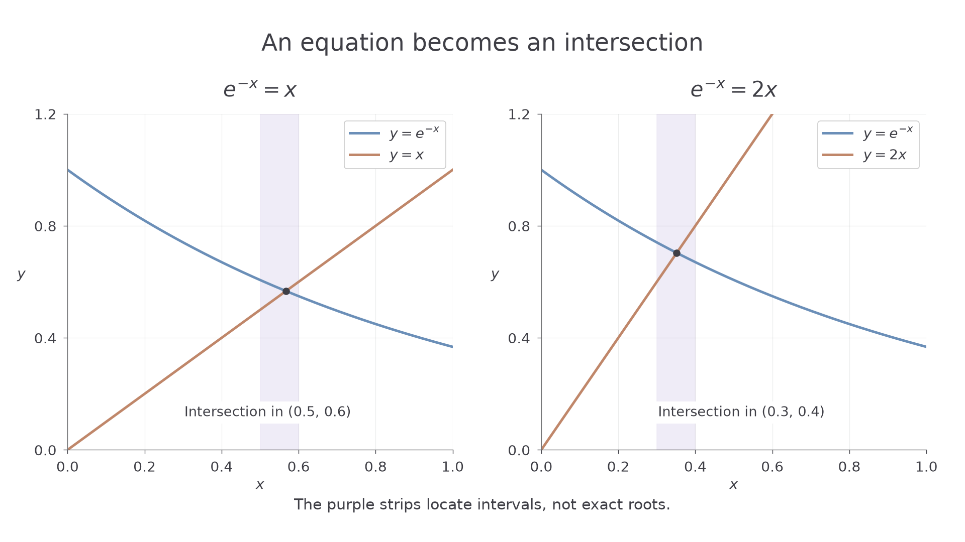
[DIAGRAM: asset_name: Intersections locate solutions; asset_slug: root-intersections; caption: Changing the line from y equals x to y equals 2x changes the intersection with the same exponential curve; description: Two coordinate plots show y equals exp minus x in blue and a rising straight line in clay. The first line is y equals x and the crossing is marked in the interval 0.5 to 0.6. The second line is y equals 2x and its crossing is marked in the interval 0.3 to 0.4. Pale vertical strips identify the two intervals without claiming exact solutions.]
Worked example 1: an exponential and a line
Question. Use a suitable pair of graphs to locate the positive root of between consecutive tenths.
Plan. Compare the decreasing exponential with the increasing line .
At , their heights are and . As increases, decreases while increases. The graph shows one intersection between and .
Answer. The root lies between and .
Check. At , ; at , . The exponential changes from being above the line to being below it.
Change only the coefficient in the line. The exponential is unchanged, so the steeper line meets it earlier.
Worked example 2: a steeper line
Question. Use suitable graphs to locate the positive root of between consecutive tenths.
Plan. Compare with .
The exponential starts at height and decreases; the line starts at and increases. Their one intersection is between and .
Answer. The root lies between and .
Check. At , . At , . The comparison agrees with the graph and the crossing occurs earlier than in example 1.
Graphs give shape as well as location. Here a strictly decreasing curve and a strictly increasing line can meet at most once: after one has crossed above the other, their separation continues to increase. That is a uniqueness argument specific to these graphs, not a consequence of seeing opposite signs alone.
Watch out
For , the zero of is not the solution. You need the two graphs' intersection, or the zero of the single graph .
Make the line steeper once more.
A sign change
A continuous curve cannot move from below the axis to above it without passing through the axis. This makes two function evaluations a powerful way to locate a root.
Sign-change argument
If is continuous throughout and and have opposite signs, then has at least one root in . If an endpoint value is zero, that endpoint is already a root.
For the functions here, continuity means the graph is connected throughout the tested interval, with no break or undefined input. Polynomials and exponentials are continuous for all real inputs. A reciprocal has a break where its denominator is zero; a logarithm requires a positive argument; tangent has breaks where cosine is zero. Check these restrictions before using signs.
Worked example 3: consecutive integers
Question. Show that has a root between and .
Plan. Evaluate the polynomial at both endpoints and use its continuity.
Let . Then
Answer. The polynomial is continuous on . Since , at least one root lies between and .
Check. The negative value at and positive value at put the endpoints on opposite sides of the axis; neither endpoint itself is a root.
Keep the equation and narrow only the interval. This is a systematic search rather than a new method.
Worked example 4: consecutive tenths
Question. Show that has a root between and .
Plan. Test the same continuous function at the closer endpoints.
Answer. Continuity and the sign change establish a root in .
Check. At the midpoint, . Testing that midpoint would narrow the bracket further to , consistent with the answer.
Continue this lesson.
You’re previewing NovaLearn without an account. Create a free account to read the rest.
Create free account