5.5 - Normal probabilities
A normal curve turns a measurement range into an area. Learn what its parameters mean, standardise measurements to use the supplied normal tables, and combine left-tail areas to find between and outside probabilities.
A continuous model
A measurement has normal distribution with mean and standard deviation . What is the chance that it lies between and ? The endpoints are different distances from the mean, so symmetry alone cannot give the answer. We will turn both endpoints into distances measured in standard deviations.
A continuous random variable models measurements which can take any real value in an interval. In a normal model, probability is represented by area under a smooth, bell-shaped curve. Its total area is , and it is symmetric about the mean.
Normal distribution
Write when has a normal distribution with mean , variance , and standard deviation .
The curve is centred at . Larger gives a wider, lower curve; the total area remains .
There is area on each side of . A single exact value has zero area, so . Consequently for a continuous normal variable. This equality does not hold for a discrete count with positive probability at .
Worked example 1: reading the parameters
Question. Given , state its mean and standard deviation. Find and .
Plan. Read the second parameter as variance, then use symmetry and the area of a point.
The line divides the curve into equal areas. A single vertical line has no area under the curve.
Answer. Mean , standard deviation , , and .
Check. The two half-areas sum to ; no extra probability is needed for the point at the centre.
Keep the mean fixed and change only the variance. The centre stays put while the spread changes.
Worked example 2: a wider distribution
Question. Given , state its standard deviation and . Compare its spread with that of .
Plan. Square-root the variance and compare standard deviations, then use symmetry.
The normal curve for is twice as wide on the measurement scale and lower at its centre. Both curves are symmetric about .
Answer. Standard deviation , ; has twice the standard deviation of .
Check. Doubling a standard deviation multiplies the variance by : . It does not double the total probability.
[DIAGRAM: asset_name: Mean and spread of normal curves; asset_slug: normal-mean-spread; caption: The two curves share a mean, while a larger standard deviation spreads the same total area more widely; description: Normal density curves N(40,9) and N(40,36) share a dashed vertical mean at 40. The narrow curve has standard deviation 3 and the wider curve has standard deviation 6. Both are symmetric and a note states total area under each curve equals one.]
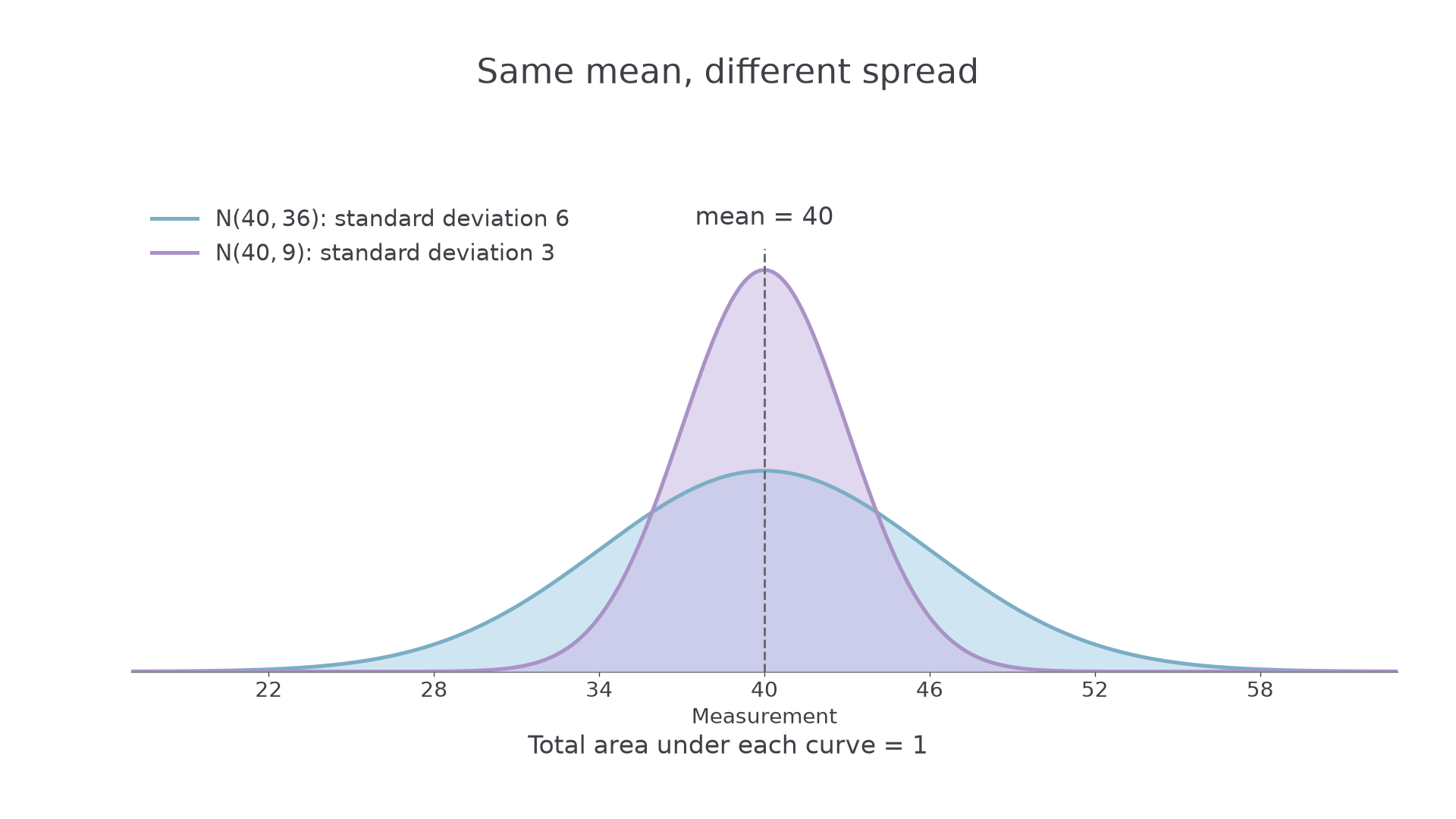
A normal curve extends indefinitely in both directions. It can be a useful model for a measurement even when the real quantity cannot be negative, provided the unrealistic tail has negligible probability in the situation. The model is an assumption to assess, not a consequence of knowing just a mean and variance.
Watch out
In , the standard deviation is , not . Curve height is not probability: probability comes from area over a range.
Check the notation before any calculation.
Standardising
Subtracting the mean tells you how far a measurement lies from the centre. Dividing by the standard deviation tells you how many standard deviations that distance represents. A value below the mean gives a negative result.
Standardising a normal variable
If , then
Not in the formula booklet as a transformation: learn it. The supplied normal tables describe .
The tables give the left-tail probability for positive . For , use row and column , giving . For a third decimal, the ADD columns supply an interpolation adjustment in units of : at , add units, giving .
For negative values, symmetry gives
This identity and the meaning of are printed above the supplied table. A right-tail probability is , whatever the sign of .
Worked example 3: a positive standardised value
Question. . Find .
Plan. Use standard deviation , standardise the boundary and read the left-tail table.
Answer. , to significant figures.
Check. The boundary is above the mean, so the left area must exceed . Also reverses the standardisation.
Reflect the boundary across the same mean. The standardised value changes sign, so the positive table entry must be complemented.
Continue this lesson.
You’re previewing NovaLearn without an account. Create a free account to read the rest.
Create free account