3.4.2.3 - Choosing and interpreting geographical graphs

Line graphs and change

Line graphs suit ordered continuous dimensions such as time or distance, where joining adjacent observations helps reveal change.

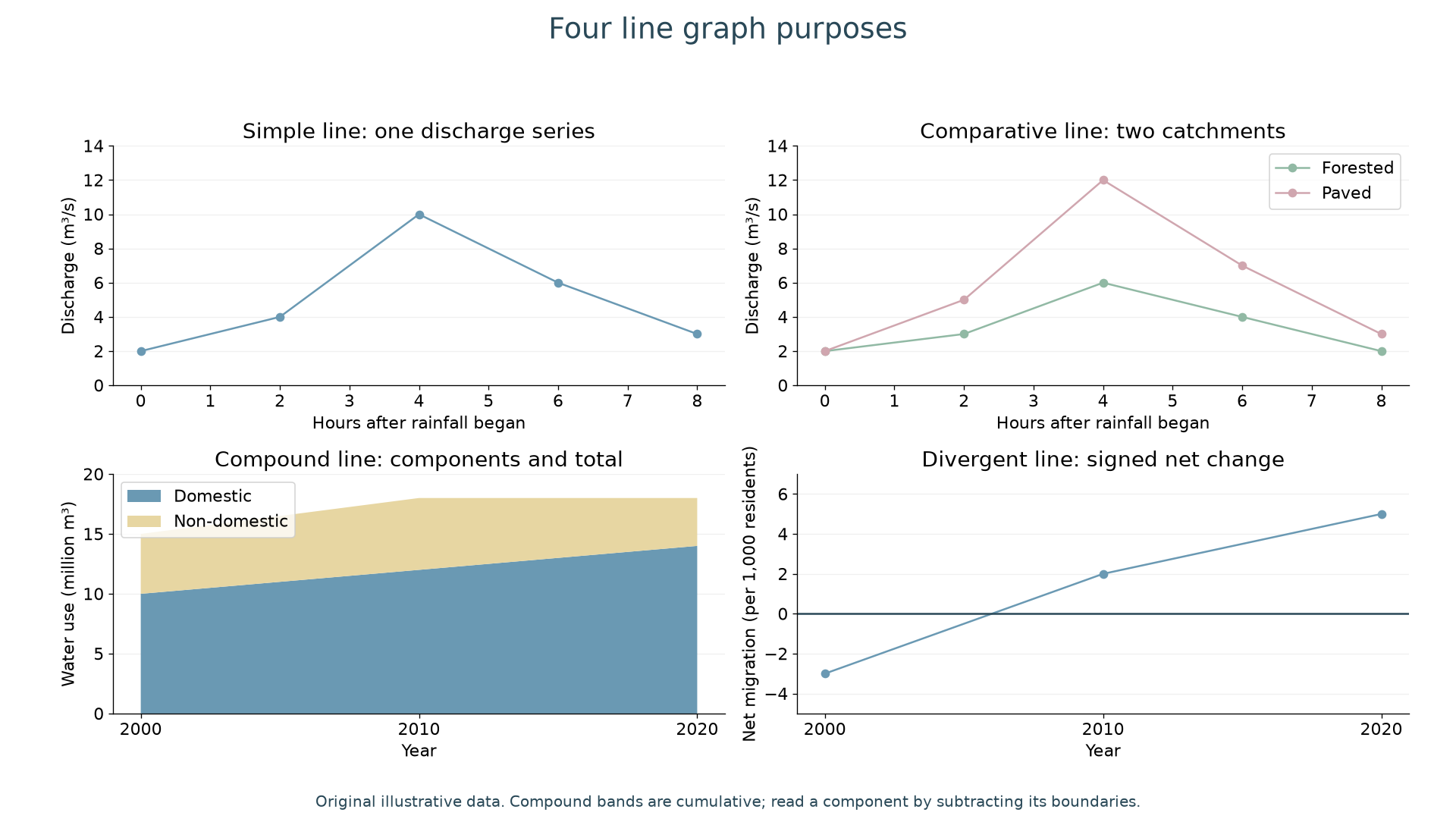
The simple line graph follows one series: discharge rises from 2 to a peak of 10 m³/s four hours after rainfall begins, then falls to 3 m³/s by hour eight. The joining segments show change between readings, not proof that every intermediate value was measured. A comparative line graph puts series on common axes: the paved catchment peaks at 12 m³/s compared with 6 m³/s for the forested catchment. Both peak at hour four. A larger peak is visible, but the graph alone does not isolate land cover from differences in rainfall, area or geology.

A compound line graph stacks related components that add to a total. In 2010 domestic use is 12 million m³, the total is 18, and non-domestic use is the difference, 6. In 2020 the same total of 18 consists of domestic 14 and non-domestic 4. Reading the upper boundary as non-domestic use would wrongly report 18. This form displays total change well, but an upper component's changing baseline makes it harder to compare than separate lines.

A divergent line graph shows signed values around zero. Net migration of −3 per 1,000 residents represents a net loss; +5 a net gain. The change from −3 to +5 is eight per 1,000, not two. Zero is meaningful and must remain visible. Negative net migration does not imply a negative population.

To construct a suitable line graph, select an ordered horizontal variable, give both axes units, use a consistent scale, plot each pair accurately and distinguish series in a key. Compound components must share units and add without overlapping definitions. For notebook practice, reconstruct one panel from its labelled values; do not join unrelated categories to imply a continuous process.

Bar graphs and categories

Bar graphs compare discrete categories using separated bars rather than implying a continuous path between them.

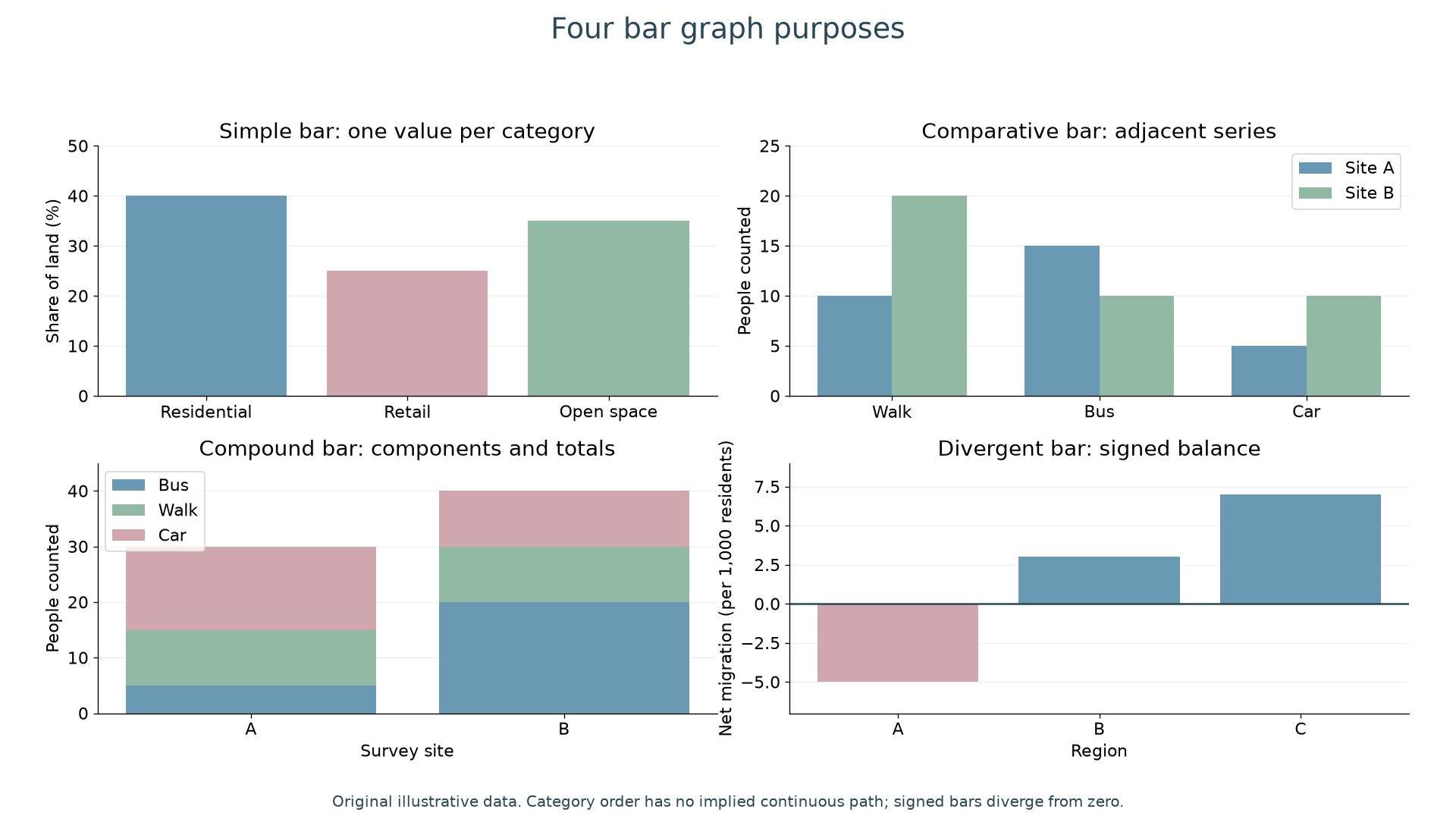
A simple bar graph presents one value per category: residential land is 40%, retail 25% and open space 35%. Equal bar widths and a zero baseline make heights comparable. A truncated baseline can exaggerate differences; if a break is necessary, make it explicit and judge its effect.

A comparative bar graph places matched series beside one another. Site B has 20 walkers against A's 10, while A has 15 bus users against B's 10. The largest category is therefore different at the two sites. A compound bar graph stacks components: site A totals 30 people and B totals 40. B's walking component is 10 people, from cumulative height 20 to 30, rather than 30. A percentage compound bar would instead make each total 100%, showing composition while concealing unequal counts unless totals are stated.

The divergent bar graph shows a balance either side of zero: region A has −5 net migrants per 1,000 residents, compared with +3 in B and +7 in C. Labels must state whether the figures are numbers, rates or percentages. A rate enables comparisons between differently sized populations; a total answers a different question.