3.1.3.5 - Coastal field measurements and spatial evidence
Choose and interpret coastal observations, measurements, maps, statistics and qualitative evidence. All practice data here are original illustrations; they are not claimed field visits or assessed investigations.
Observation and spatial design
A useful observation records what was seen, where and when, while separating that record from an explanation.
“Fresh fallen blocks lie below the cliff” is an observation; “a storm caused the failure” is an inference needing event evidence. Annotated photographs and field sketches can record scarps, sediment, vegetation, structures and access, with direction, date, tide and a scale where possible. Repeat viewpoints improve comparison. Photograph framing can hide part of the coast, so note the view rather than treating it as a complete survey.
Define a bounded question and response variable before selecting sites. To compare sediment near and beyond a defence, use several positions in each relevant zone and a consistent method. Systematic sampling at fixed intervals reveals a transect pattern; stratified sampling covers distinct exposure or management zones; random positions can reduce selection bias within those zones. Convenience access can skew the sample. Nearby sites are spatially connected, so many particles at one site are not many independent coastal sites.
Record coordinates and their coordinate reference system. A British National Grid pair uses eastings and northings in metres; latitude/longitude uses angular coordinates and needs a stated datum. Plot points or survey lines with orientation, scale and legend; do not mistake a professional survey line's endpoints for the observed cliff edge. GIS can overlay geology, management boundaries and dated change, but layers must share compatible reference systems and resolution. Old aerial imagery, tide-dependent waterlines and cliff-top lines measure different shoreline proxies.
Measuring profiles and sediment
A beach profile measures elevation along a fixed cross-shore line, making its reference point and segment geometry essential.
With ranging poles and a clinometer, measure the angle between equal-height sighting points and the segment distance. If the tape follows the sloping segment, vertical change is distance multiplied by the sine of the angle; if the measured distance is horizontal, use its tangent. State which distance was measured. Fix a sign convention, use a stable benchmark and compare repeated surveys at equivalent positions and datums. Unequal pole sighting heights need a correction; changing the start point can create an artificial profile difference.
Here is sloping tape distance in metres, the segment angle, and signed vertical change in metres.
In original illustrative data, two landward segments have sloping distances 10 m at +4° and 8 m at +6°. Their rises are m and m, giving 1.534 m total above the start. Their horizontal spans are about 9.976 m and 7.956 m. A plotted profile needs these horizontal positions, not tape distances silently treated as horizontal.
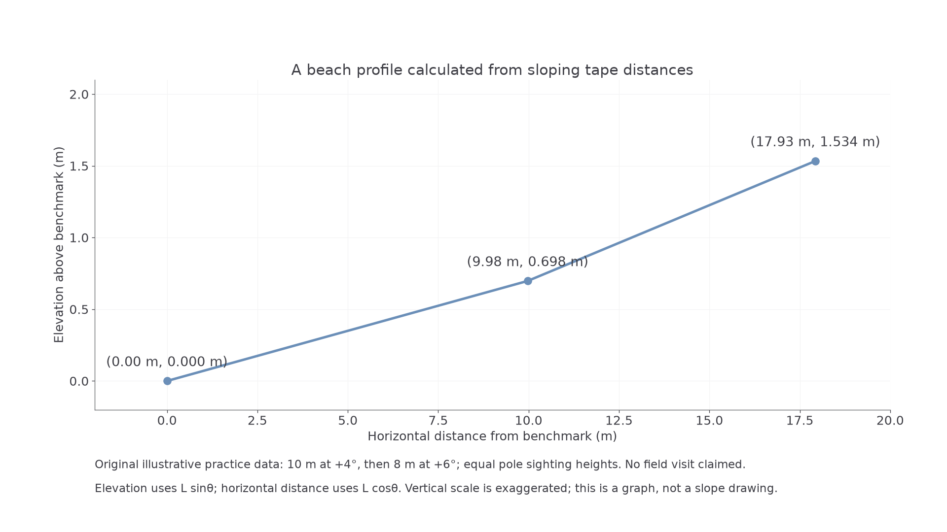
The illustrative graph exaggerates vertical scale, so its visible slope must not be read as the measured angle.
Sediment sampling can measure intermediate-axis size with a ruler/calipers, and describe roundness using a stated scale. Use a consistent selection rule, sample count and zone; choosing only the largest visible stones biases size upward. Repeat readings, calibrated instruments and documented tide/weather improve reliability. They do not eliminate systematic selection bias or make hazardous cliffs safe. Real field activity follows the centre's risk assessment, permissions and tide/weather planning; never approach unstable cliff edges or work in unsafe surf to obtain a sample.
Continue this lesson.
You’re previewing NovaLearn without an account. Create a free account to read the rest.
Create free account