3.1.2.5, 3.1.2.6 - A hot desert setting and field evidence

Death Valley: observing a connected landscape

Death Valley is a mid-latitude hot-desert basin in California's Mojave region. Mountain barriers restrict moisture supply; tectonic relief provides steep slopes and sediment sources. Weathering and mass movement supply debris, episodic water cuts channels and deposits fans, and wind reworks suitable sediment into dunes. Badwater's closed drainage favours fine-sediment and salt accumulation. The NPS geology account provides the setting; it does not establish that every specified aeolian landform occurs there.

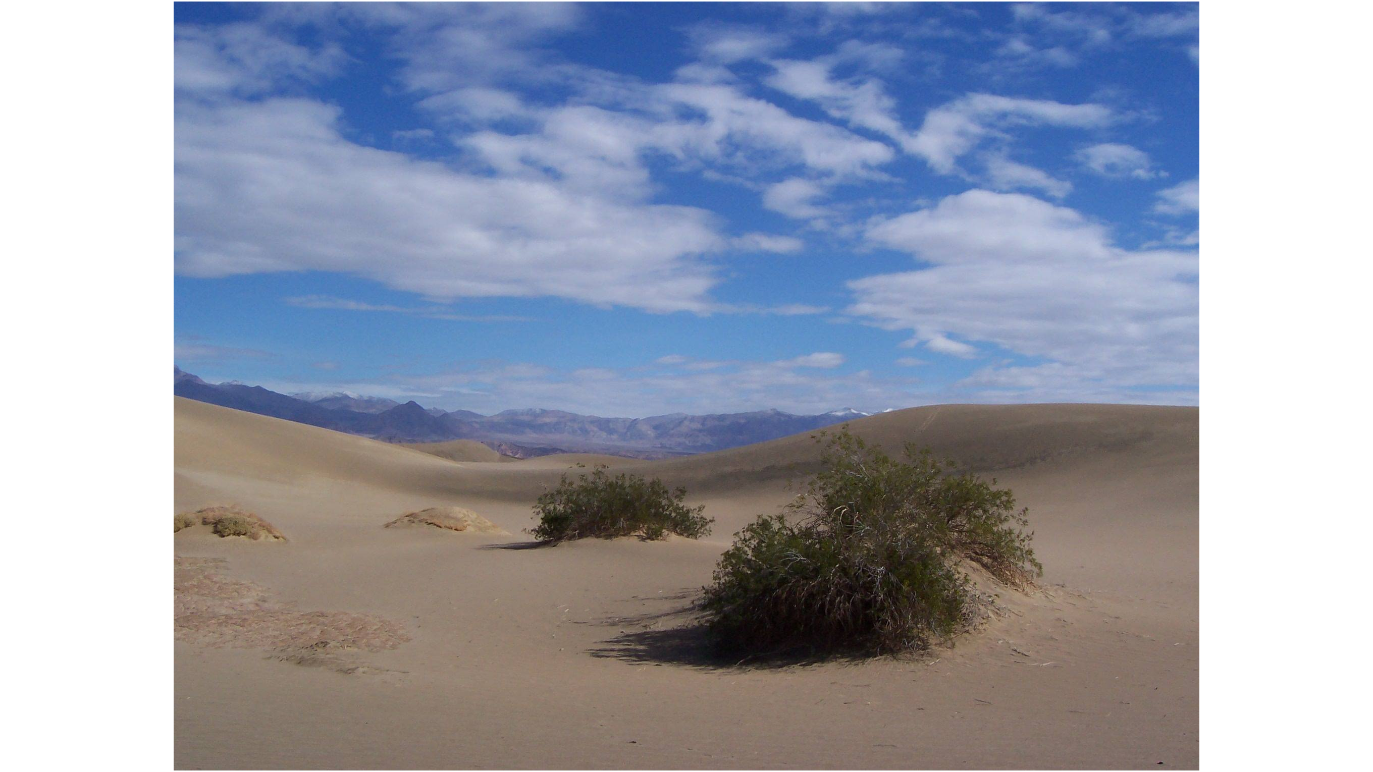
NPS public-domain photograph, 3 March 2015. Observe the dune surface and patchy plant cover before inferring processes. This photograph does not supply wind speed, migration rate or a representative vegetation percentage.

A field sketch selects relevant visible outlines and labels: slope breaks, crest, exposed sand, plants and surrounding relief. Record viewpoint, orientation, date and scale where known; mark missing information as unknown. Separate observation ('sand exposed between plants') from inference ('plants may trap moving sand'). Repeated photographs from a fixed viewpoint strengthen evidence of change, while one attractive image cannot establish frequency or cause.

Actual published measurements at Dumont Dunes

Dumont Dunes is a separate Mojave site, not Death Valley National Park's Mesquite Flat dune field. Draut and Rubin's USGS 2007 report includes a 16-hour trial in late February–early March 2004 on Dumont's northern sand sheet. Wind sensors at 0.3, 1.0 and 2.0 m sampled at 1 Hz, with 10-second averages stored. Wind-vane sediment traps at 0.1, 0.4, 0.7 and 1.0 m stood about 5 m from the sensor tripod. Height matters because transport varies vertically, and a turning trap better faces changing wind.

The report gives mean wind at 2 m as 3.6 m/s and maximum gust as 10.8 m/s. Its 61.8 g captured-transport estimate integrates the profile from 0–1 m. A dry unobstructed surface and finite duration bound the result: this is neither a whole-desert annual flux nor a measurement of all suspended dust. Trap width, exposure time, sampling interval and efficiency must be recorded to compare trials fairly.

Estimated trap efficiencies of 105–115% imply possible overcollection. Divide observed mass by the efficiency factor: 61.8 ÷ 1.05 ≈ 58.9 g, and 61.8 ÷ 1.15 ≈ 53.7 g. The corrected range is therefore about 53.7–58.9 g. This is an instrument-correction range, not variation among repeated independent samples. Source: USGS Open-File Report 2007-1001, Methods/Figure 15/Table 5.

Manipulating data and descriptive statistics

Preserve raw data, units and missing values before deriving summaries. Convert consistently, identify outliers without silently deleting them, and distinguish an average wind value from gusts. A model-to-measured transport ratio of 1 means agreement; ratios below 1 underestimate, above 1 overestimate. Dumont Table 5 reports raw ratios of 0.856 for Kawamura and 34.9 for Williams; those show very different agreement, without proving one model is best at every site.