3.4.2.1, 3.4.2.5 - Field sketches, photographs and remote sensing

Photographs, sketches and diagrams

A useful visual annotation separates a visible observation from an explanation inferred using other knowledge.

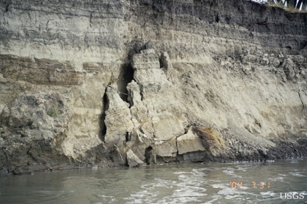
USGS Personnel, Bank Erosion: right bank of the Missouri River southwest of Brockton, Montana. USGS source, public domain. The source page does not establish a precise observation date; do not use this single photograph to calculate a rate.

The photograph shows an exposed bank face, cracks and detached or partly detached material above the water. An annotation might point to a crack and state “fracture separates a block from the bank”. “Bank instability may be producing collapse” is an inference. The image does not show when the crack formed, how far the bank retreated or whether a flood triggered the movement. Apparent sizes vary with distance from the camera; without a reliable scale and camera geometry, pixel length is not ground length.

A field sketch deliberately selects relevant features from a field view. Establish the major outlines and foreground/background relationships, then add sparse annotations linked by clear leader lines. Record viewpoint, direction, place, time and an appropriate scale or “not to scale”. Omit decorative detail without omitting evidence that challenges your interpretation. Preserve the relationship between water, bank face and material at its foot; do not invent a feature hidden outside the view. Two people may emphasise different features, so a sketch is a reasoned representation rather than a neutral copy.

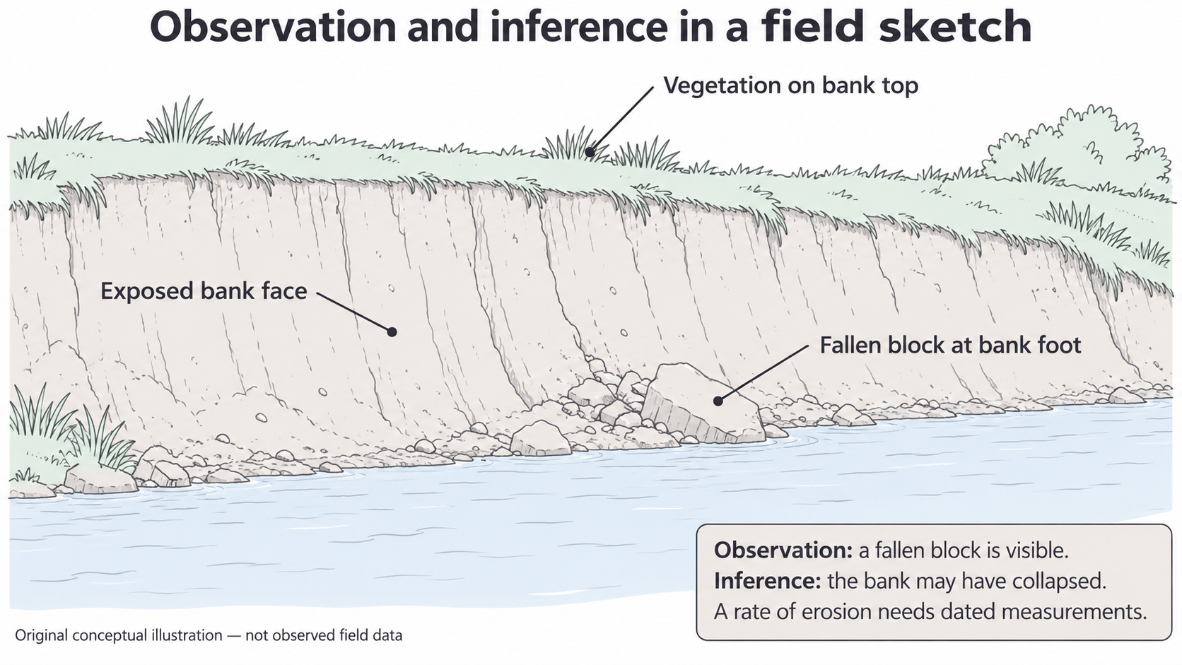
This original conceptual illustration is not a drawing of the USGS site or observed field data. It demonstrates selective annotation; its vegetation and block arrangement cannot be used as facts about the photograph.

A diagram may abstract a process further. A diagram of bank collapse can identify gravity, weakening and movement through arrows, while a field sketch primarily records spatial evidence. Read the title and arrow key: a flow arrow, a movement arrow and a leader line make different claims. Add a process annotation only when it explains a mechanism supported by the taught model; do not convert every label into a causal claim. An illustrative diagram cannot independently prove that the depicted process happened at a particular place.

Sketching and annotation in a notebook are useful ungraded construction practice. Written checks here assess how well you interpret visible evidence and justify annotations, rather than awarding a drawing mark through prose.

Annotating graphs with evidence

A graph annotation should point to a pattern or feature and explain it using the graph's actual variables, units and sampling conditions.

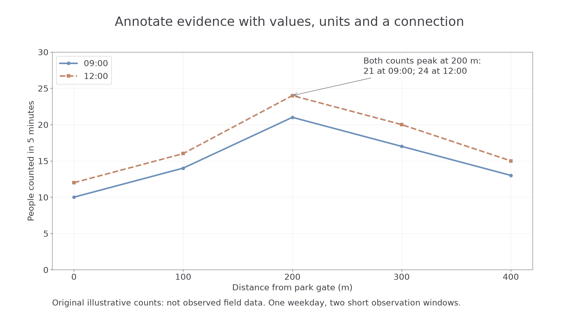
Original illustrative counts, not observed fieldwork. Each point is a five-minute count at a stated distance from a park gate; the two series represent 09:00 and 12:00 on one training weekday.

Start with the axes and key. Distance is in metres, not elapsed time; the vertical axis is people counted in five minutes, not total daily park visitors. Both series rise from the gate to a peak at 200 m, then fall. At the peak, the counts are 21 at 09:00 and 24 at 12:00. The midday series is higher at every sampled distance, but its difference from the earlier count varies between two and three people. These are connected comparisons rather than a list of point readings.

An annotation “shared maximum at 200 m: 21 and 24 people per five minutes” connects location, values and pattern. “The café attracts everyone” is not shown by these axes: it requires a mapped café and evidence about motives. Mark an anomaly only if it departs from a stated pattern. Do not add a “line of causation” because two series vary together.

Check the axis baseline and intervals before assessing the size of differences. A truncated vertical axis can make a small count difference appear large. The joining lines help read the sequence; they do not supply continuous observations at every metre. A bar, scatter or line graph uses different conventions, so decide what the marks represent before annotating. A sharp change may be real or reflect the time, method or location of sampling.

Retain the original values and provenance when annotating digitally. Text boxes should not cover data or change a scale. Notebook graph construction is ungraded here; supplied-graph interpretation is markable. A supported written conclusion for this dataset is that counts were higher at midday at these five sites during these brief windows. It does not establish a general weekly pattern without repeated sampling.

Geo-located and digital imagery

Digital imagery becomes more useful geographically when its location, direction, time and processing history are known.

A digital image is stored electronically. Geo-located imagery has a location attached, for example a GPS-tagged ground photograph; geospatial imagery relates the positions of features or pixels to a spatial reference so it can be compared with maps. A photograph taken at one GPS point is not automatically an orthorectified overhead map. The camera position is different from the positions of all objects in its view.

For a repeat photographic enquiry around your study centre, define the feature to compare, such as the condition of a public riverside bank or a street frontage. Select safe public viewpoints, record a site ID, camera location, viewing direction, date/time and conditions, and retain an unchanged original file. Repeat from the same position, height, direction and approximate framing. Obtain permission where needed and avoid identifiable people or private interiors. A stable landmark helps check alignment; a GPS tag alone may have positional error and says nothing about which way the camera faced.

Metadata describe the image: capture date, device, coordinates and processing. A copied or edited image may lose metadata; a device clock may be wrong. Verify important details against a field log rather than treating the filename as proof. Cropping can hide evidence outside the frame; contrast enhancement can emphasise a feature without creating a new observation. Record edits and distinguish an original from a processed working copy.

For a training comparison, an apparent increase in paving between two photographs could arise because the second camera was turned further right. Repeating the viewpoint and annotating stable boundaries reduces that ambiguity. It does not remove seasonal differences, occlusion by vehicles or changes in lighting. Combine the photographs with a base map and an independently recorded surface classification before claiming the fraction of the whole area that changed.

Your own enquiry needs locally appropriate viewpoints and safeguarding, rather than adoption of the Missouri photograph as your fieldwork. This method teaches evidence collection; it does not create observations or a completed assessed investigation.

Remote sensing, resolution and change

Remote sensing measures the surface from a distance, allowing extensive or repeated spatial evidence to be studied with explicit limits.

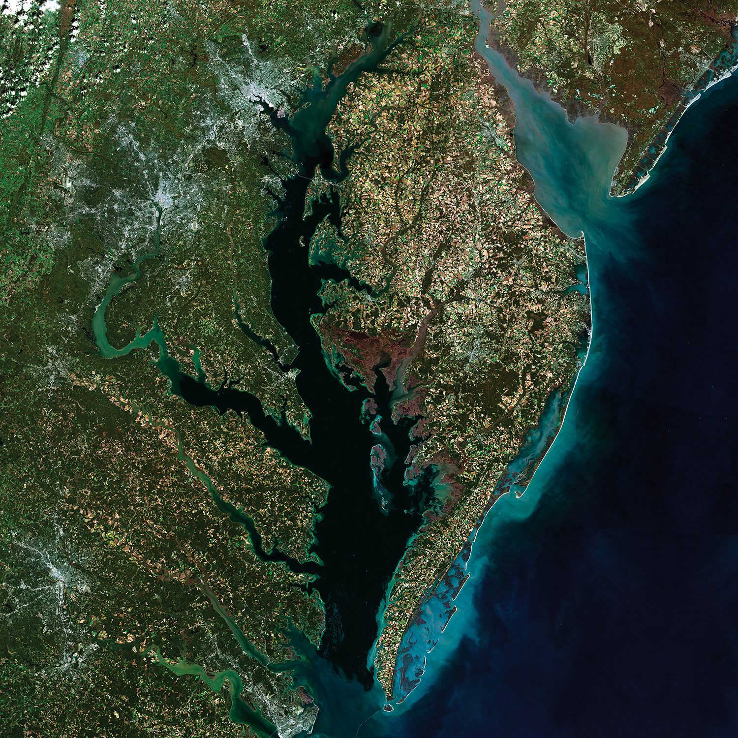
USGS EROS, Chesapeake Bay: A Landsat 8 Surface Reflectance Mosaic, public domain. Source, published 23 October 2018; five scenes acquired in October–November 2014. This is a true-colour mosaic rather than a single instant. The embedded display has no measurement scale: do not measure ground distance from its screen size.

The broad water body, branching inlets and surrounding land are visible. Annotate their relationships before attaching an explanation. Dark water does not prove cleanliness, and a green patch is not sufficient evidence of a named species. A true-colour image combines visible bands to resemble human vision; a false-colour composite assigns other bands to display colours, so red may represent vegetation rather than fire. Always read the band combination or key.

Spatial resolution is the ground area represented by a pixel; temporal resolution concerns how frequently comparable observations are available; spectral resolution concerns the wavelength bands distinguished. USGS Landsat surface-reflectance products have 30 m spatial resolution. One square 30 m pixel represents 900 m². A narrow strip of vegetation and adjacent paving may both contribute to that pixel's signal, so displaying it at a larger size creates no finer ground detail. A derived map may assign one class to a mixed pixel: classification is an interpretation that needs validation.

A controlled change comparison

Original illustrative training classifications use the same 16 square 30 m pixels on two dates, with vegetation defined identically. Twelve pixels are classified as vegetation on date1 and nine on date2. Vegetation cover changes from 75% to 56.25%: a reduction of 18.75 percentage points, equivalent to 2,700 m² in this 14,400 m² training extent. This is net change; some pixels could gain vegetation while others lose it. It is not a real satellite observation or evidence of a particular development.

For actual change detection, align images to the same spatial reference and extent, use comparable resolution/bands and classification definitions, and inspect cloud/shadow and seasonal differences. A cloudy pixel is missing/obscured evidence, not zero vegetation. Mask such pixels and use a common valid area for comparison, stating the exclusions. Check some classifications against suitable dated ground evidence. A mosaic's different acquisition dates matter when the change is rapid.

Remote imagery can extend spatial coverage beyond accessible field sites; ground photographs can explain details and test a class. Neither should be treated as complete truth. A defensible annotation states the observed pattern, the relevant date/resolution and a qualified interpretation, while identifying the evidence needed to test it.