3.4.1, 3.4.2.1, 3.4.2.2, 3.4.2.5 - Maps, spatial data and GIS in geographical enquiry
Maps connect evidence to location. Learn to collect usable spatial records, combine layers, read scale and relief, and choose maps that represent quantities, distributions and movement faithfully. The Aster examples are original illustrative geography, not observed fieldwork or a real place.
Geographical data and GIS
A geographical record links an attribute to a location so that spatial relationships can be investigated.
Geographical information system
A GIS stores, combines, queries, analyses and presents data linked to locations. An attribute is information about a feature, such as a river measurement or a neighbourhood population.
A temperature of 18°C alone tells us little geographically. Add the sensor's location, observation time, measurement height and method, and we can compare it with other sites. A place name, address, coordinate or mapped boundary can provide the location; not all geographical data start as GPS points.
GIS commonly represents vector data as points, lines and polygons: individual sensors, roads and neighbourhood areas. Raster data divide space into cells, each holding a value, such as elevation or a satellite-derived land-cover class. Raster cells summarise areas; a point symbol need not describe the surrounding cell. A coordinate reference system defines how coordinates relate to positions. Layers using different systems must be correctly transformed before comparison, rather than assumed to align because both contain numbers.
From collection to an interpretable map
For a training enquiry, “Do impermeable surfaces occur close to the Aster river?”, create a digital table with one row per site: site ID, local easting, local northing, date/time, surface class, method and uncertainty. Record a GPS position at the feature being measured, check it against a recognisable mapped feature and retain the reported accuracy. A position recorded inside a building or beside a tall wall may be displaced. Store units consistently and distinguish missing observations from zero values.
Import the table as points using its stated coordinate system. Join a second table to the points using unique site IDs, checking for duplicates and unmatched rows. A join by site name alone may confuse two sites with the same name. Overlay the river and land-cover polygons, then query sites within a stated distance or calculate each site's distance to the river. A buffer is the area within a chosen distance of a feature; it identifies proximity, not flood risk by itself.
Present the result with a title, date, key, orientation and suitable scale. Inspect implausible positions and units before interpreting a pattern. “Three sampled paved sites lie within 100 m of the river” describes the records; it does not establish that all riverfront land is paved or that paving caused flooding. GIS makes analysis reproducible when source files, transformations and query choices are retained.
Base maps, scale and location
A base map supplies the locational framework against which new evidence is recorded and interpreted.
A base map shows reference features such as roads, rivers and boundaries. A sketch map selects the features relevant to an enquiry rather than copying every detail. Keep their relative positions sensible, add a north arrow and key, and state “not to scale” unless distances have been controlled. An annotation should locate a relevant observation and explain its meaning: “paved yard beside river” is more useful than “yard”.
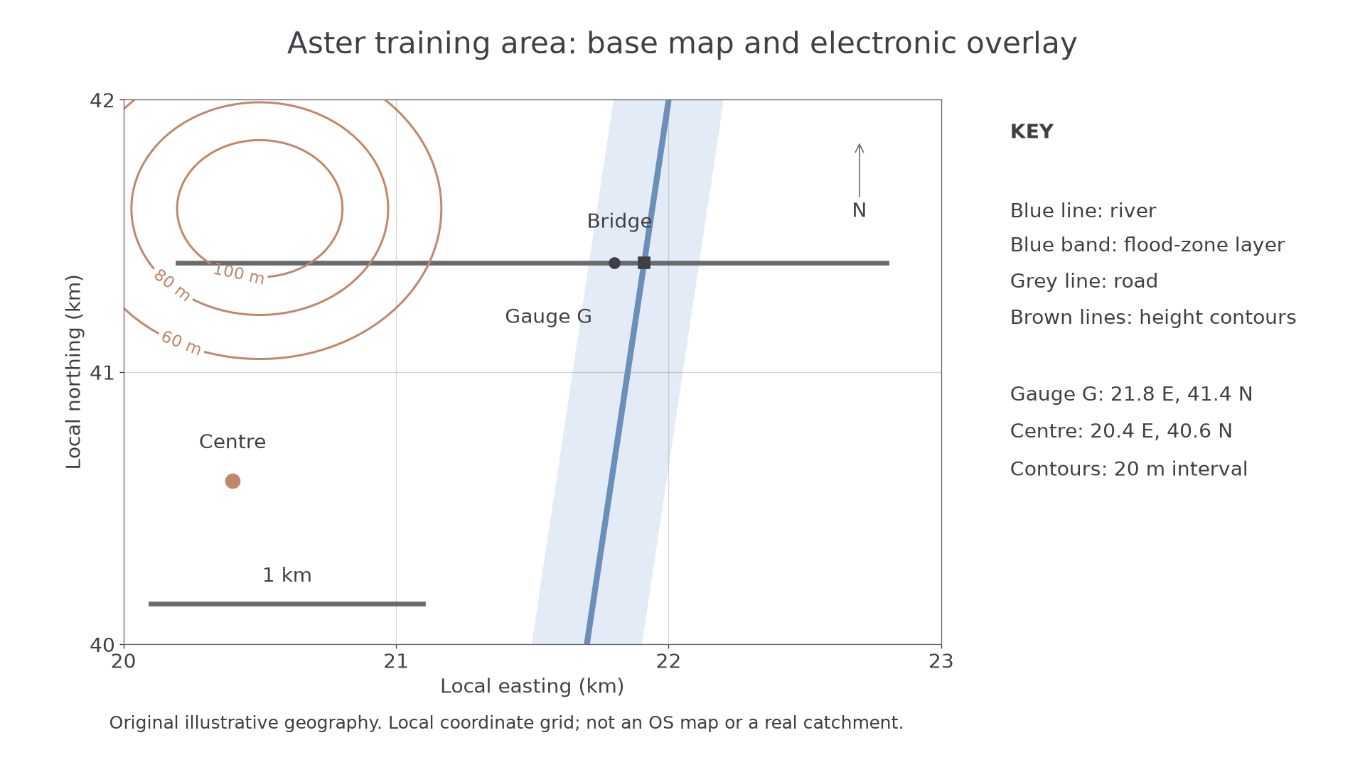
Aster's original training map uses kilometre coordinates. It is not an OS map; the blue band is an illustrative layer, not a flood prediction.
The gauge is at easting 21.8 km, northing 41.4 km. Read east first, then north. In a kilometre-grid exercise, its four-figure square reference is 2141, while tenths within that square give 218414. A six-figure reference identifies a 100 m square, rather than proving metre precision. On a real British National Grid map, include the correct two-letter 100 km square identifier; these fictional local coordinates have no such letters. The Ordnance Survey map-reading guide explains the official grid and symbols.
A large-scale map shows a smaller area in greater detail. At 1:25,000, 1 cm represents 250 m; at 1:50,000 it represents 500 m. Thus a 6 cm route is 1.5 km on the first map and 3 km on the second. Use a ruler for a straight distance; trace a curved route with a strip of paper or suitable digital measuring tool. When a digital image is resized, a printed ratio may cease to match the screen, while a scale bar resized with the map remains useful.
OS Explorer and Landranger maps therefore support different levels of enquiry detail. Consult their actual keys: symbols are conventions, not pictures whose meaning should be guessed. Contours join equal heights; close spacing indicates a steeper slope where the height interval is the same. Trace relief and drainage together before inferring a catchment boundary. A road crossing a river does not establish a watershed.
A useful field map annotation links position, measurement and conditions: “G: depth 0.42 m, 10:15, method M1”. The number does not become reliable merely because it is on a detailed map.
Overlays and a local enquiry
An overlay reveals how two spatial distributions coincide when their locations, dates and definitions can be compared.
For a physical overlay, trace one theme onto transparent material, mark reference points and align it over a base map at the same scale and orientation. A pencil mark that shifts when the sheet moves is not evidence of geographical change. An electronic overlay combines layers in a GIS, retaining their coordinate systems and attributes. Turning layers on and off helps distinguish a genuine relationship from a cluttered display.
In Aster, the blue flood-zone band crosses the road, while the study centre lies outside the band. That supports a question about whether access could be interrupted; it does not show the timing, depth or probability of any flood. Add elevation, drainage and a dated risk source before making a stronger claim. Boundaries and mapping choices shape the apparent overlap: an old flood layer may be inappropriate for a new engineered channel.
Adapt the method to your own study centre
Choose a feasible, small enquiry such as whether paved surfaces cluster near a local stream. Obtain a lawful current base map and record its source, scale and coordinate system. Define the study area and surface categories before collecting data. At safely accessible predetermined sites, record the surface category, location, time and method; collect no unnecessary personal information. Digitise the river, add the sites and compare their positions with a stated buffer. Check suspicious points in the field or against a second source. Explain that accessible sites may omit private or dangerous land, so the mapped pattern represents the sample, not necessarily the whole area.
The complete Aster workflow illustrates how to make a map; it is not a substitute for your own local observations or an independent investigation. If there is no suitable stream, retain the logic but ask a justified human-place question, such as the distribution of tree cover around the centre. Adapt the variable, safe access, sampling frame and comparison distance to that setting.
Spatial coincidence is evidence to investigate. A defensible explanation also needs appropriate dates, definitions, coverage and process knowledge.
Mapping magnitude and spatial pattern
The map type should match whether the variable is a total at a location, a rate over an area, a distribution of occurrences or a continuous surface.
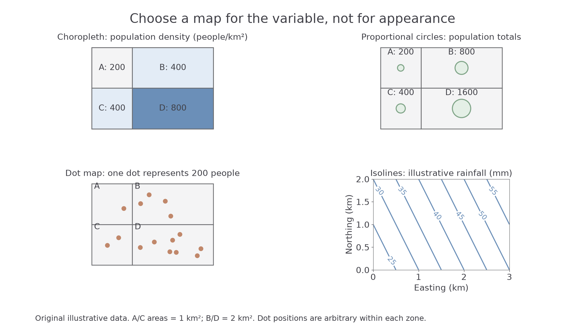
The same illustrative population is represented differently. All positions and values were plotted from the stated training data; the rainfall panel is a separate continuous variable.
| Zone | Area (km²) | Population | Density (people/km²) |
|---|---|---|---|
| A | 1 | 200 | 200 |
| B | 2 | 800 | 400 |
| C | 1 | 400 | 400 |
| D | 2 | 1,600 | 800 |
A located proportional-symbol map places a symbol at its relevant location and varies its area with the total. D has eight times A's population, so D's circle must have eight times its area. Circle area is proportional to radius squared; its radius is therefore , about 2.83, times A's. Doubling the radius quadruples area. Check the key and whether the symbol is positioned at a town, representative area centre or exact observation site; these are different geographical claims.
A choropleth map shades whole areas by class. For comparisons between differently sized zones, use a suitable rate or density: B has twice C's population but also twice its area, so both have 400 people/km². Shading by totals could wrongly suggest B is more densely settled. Class boundaries can exaggerate a small difference across a threshold or hide variation within a class. Uniform shading does not mean everyone in a zone experiences the same conditions.
A dot map uses a fixed quantity per dot. At 200 people per dot, A has one and D eight. Dots can reveal concentrations when placed from suitable detailed evidence. Here they are positioned arbitrarily within zones, so they do not identify homes; changing the dot value or placement rules can change the visual impression.
An isoline map joins equal values on a continuous surface, such as rainfall, temperature or height. In the training rainfall panel, values increase towards the northeast. A value between two lines must be estimated and its precision limited by the contour interval and observations used for interpolation. Do not use isolines to imply that a categorical variable, such as nationality, changes smoothly.
To create these maps in ICT, select the correct attribute and units, choose an appropriate projection, use proportional areas or explicit choropleth classes, and supply the key and source period. Test a known value against the display before interpreting the pattern. Construction in your notebook or GIS is useful practice; assessed answers here interpret supplied maps and explain choices.
Flow, desire and trip lines
Movement maps distinguish how much travels between places from where individual journeys actually go.
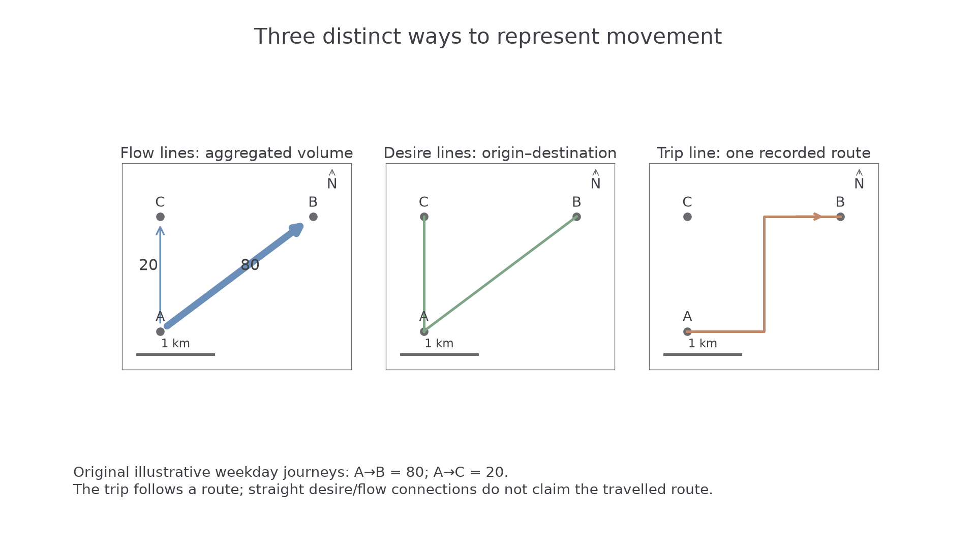
All three panels use the same original local positions. They represent different claims about illustrative weekday journeys.
A flow-line map shows aggregate movement, with direction and line width or a labelled volume. The flow from A to B is 80 journeys, compared with 20 from A to C: four times as many. A connecting line may be schematic, so it must not automatically be read as the route taken. Check units: tonnes per year and journeys per weekday are not comparable flows.
A desire line connects an origin to a destination directly, regardless of the route. It reveals a connection and can be weighted by demand. It does not show that a traveller crossed every intervening property or followed a straight road. A trip line traces an actual recorded journey route. In the final panel, the turn through the road network adds distance compared with the direct A–B line. Several recorded trips can reveal route use, but a small GPS sample does not establish everybody's behaviour.
When interpreting movement, identify origins, destinations, direction, magnitude and recording period before explaining connections. A transport route may enable travel, but the map alone does not identify employment, cost or personal motives. Aggregate or anonymise individual trip data; precise repeated start/end points can reveal homes and workplaces even when names are removed.
Atlas and weather-map evidence
Atlas and weather maps support different scales of explanation, so their purpose and conventions must be read before their patterns.
An atlas map can locate an unfamiliar region, compare latitude, relief or climate and place a local enquiry in a wider setting. Use its title, key, coordinate grid, scale and source date. A world political map will not show the stream beside a study centre. Map projections transform the curved Earth onto a flat surface, so world maps can distort area, shape, distance or direction; an apparent size comparison may require an equal-area map. A physical map helps test whether an inferred route crosses high relief, while a thematic climate map describes a different variable at a stated averaging period.
A synoptic chart summarises atmospheric conditions over a broad region at a stated time. Isobars join equal air pressure, usually in hectopascals (hPa). A low-pressure centre is labelled L, a high-pressure centre H. Closer isobars indicate a stronger pressure gradient and generally stronger winds; they are not contours of land height. Fronts mark boundaries between air masses. Triangles on a cold front and semicircles on a warm front indicate its movement direction. The Met Office guide provides an authoritative example of these conventions.
For an original training chart with successive 1004 and 1008 hPa isobars, compare their distance apart in two regions. If the same 4 hPa change occurs over 100 km near P but 400 km near Q, the gradient is stronger near P. This supports a stronger-wind inference near P, not an exact wind speed or proof that P has more rainfall. Rain depends on moisture, uplift and other conditions; the chart's fronts provide additional evidence. Check whether a chart is an analysis or a forecast, and compare the same valid times before claiming change.
For a local catchment enquiry, use atlas relief/climate as context, a dated synoptic chart for broad weather conditions and a local rainfall record for the actual measured input. Combining scales can strengthen explanation, provided a regional pattern is not presented as a precise reading at an unmeasured site.