4.4(b)–(c) - Correlation and Spearman’s rank

Scatter graphs and correlation

A scatter graph plots paired observations: each point represents two measurements from the same case. For example, each site may have a distance from a river mouth and a median sediment diameter. Labelling the axes with variables and units makes the pairing interpretable; independently sorting the two columns before plotting would destroy the original relationship.

Positive association means that higher values of one variable tend to occur with higher values of the other. Negative association means higher values tend to occur with lower values. Weak or absent association means that one variable provides little consistent information about the other in the observed sample. Strength concerns how consistently the points follow a relationship, not whether the slope is steep. A narrow vertical scale can make an identical relationship look steeper without changing the data.

A linear relationship approximately follows a straight line. A monotonic relationship consistently increases or decreases but may curve. If illustrative values are $x=1,2,3$ and $y=1,4,9$, their ordering is perfectly increasing even though a straight line does not pass through all three points. Spearman's rank measures monotonic association by comparing order rather than measuring the slope in the original units.

Examine the whole plot. A single unusual observation may alter an apparent trend, and two clusters can reflect different underlying populations. An average relationship may conceal local departures caused by geology, defences or tributaries. Those departures can be geographically important rather than mere noise to delete. Check a suspected recording error against original records before removing it, and explain any exclusion.

Worked increasing pairs

Illustrative soil observations pair vegetation cover of 10%, 20% and 30% with moisture of 8%, 13% and 19%. Keep each site's pairing when plotting:

Label cover on the horizontal axis and moisture on the vertical, with percent units. The points rise from left to right, showing positive association; the plot alone does not isolate a vegetation effect.

Worked decreasing pairs

Illustrative air-quality observations pair road distances of 2, 5 and 8 metres with particle concentrations of 70, 62 and 54 micrograms per cubic metre:

Plot distance horizontally and concentration vertically without independently sorting columns. The downward pattern shows negative association, with original units retained. Wind and traffic conditions remain possible influences.

NOAA's Mauna Loa atmospheric carbon-dioxide record, begun with Scripps measurements in 1958, illustrates why variables with trends need careful comparison. Its long record contains seasonal fluctuations as well as sustained accumulation. Pairing carbon dioxide with another rising time series might yield association even where a direct causal mechanism has not been established. Temporal dependence and other changing conditions must be considered alongside a coefficient.

Lines of best fit and residuals

A line of best fit summarises a roughly linear relationship without joining successive points. For a graphical estimate, position the line through the main trend with a reasonable balance of points above and below; do not force it through the origin unless the relationship and evidence justify that constraint. A fitted regression line follows a specified mathematical criterion, commonly minimising squared vertical residuals, and need not be identical to a hand-drawn estimate.

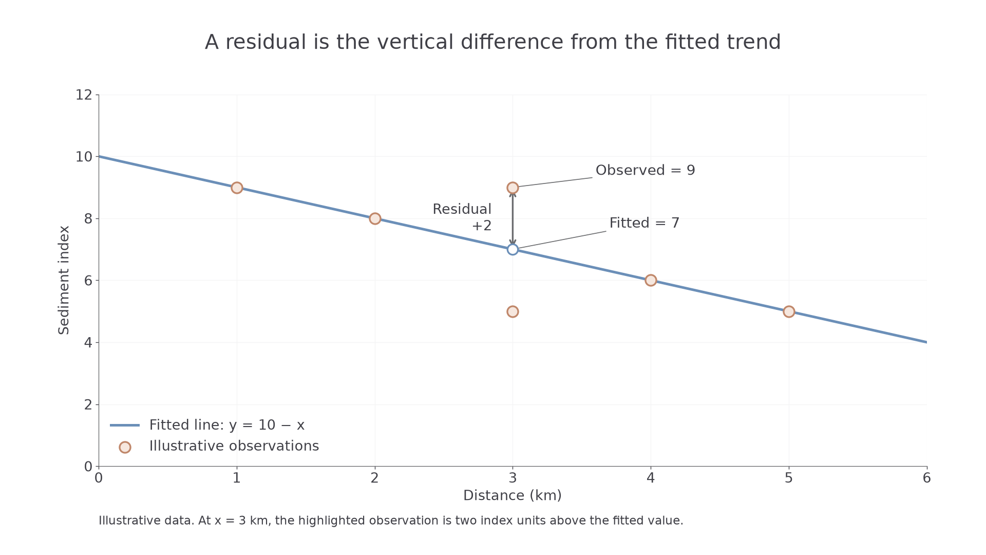
A residual is an observed value minus the value predicted by the line at the same horizontal coordinate. Positive residuals lie above the line and negative residuals below it. Small scattered residuals support a linear summary; a systematic curved pattern suggests the line is missing structure. Residual size has the units of the vertical variable, unlike a rank-correlation coefficient.

Worked positive residual

A supplied line is $y=10-x$, with distance $x$ in kilometres and a sediment index $y$. At $x=3$, the observed index is 9. Substitute the distance and subtract fitted from observed:

The point lies above the trend; a local sediment supply could explain it.

Worked negative residual

A supplied soil-moisture model is $y=4+3x$, where $x$ is vegetation-cover class and $y$ moisture percentage. At class 2, the observation is 8%:

The observation lies below the fitted value. A residual has the vertical variable's units; it is not a relative percentage change.

[DIAGRAM: asset_name: A fitted trend and a geographical residual; asset_slug: h481_s05_fit; caption: A residual measures the difference between an observation and the fitted value at the same distance.; description: An illustrative graph plots distance zero to six kilometres against a sediment index, with the supplied fitted line y equals ten minus x. At distance three kilometres an observed index of nine lies above a predicted index of seven; a vertical segment marks the residual of plus two.]