1.2 - Water and carbon as Earth systems
Water and carbon support life while moving between stores in the land, oceans and atmosphere. This lesson explains why they matter, how system boundaries change the meaning of inputs and outputs, and how to compare global stores and calculate their changes without confusing stocks, flows or units.
Water, carbon and life
Water and carbon are fundamental to living organisms, but they perform different functions.
Liquid water acts as a solvent in which many biochemical reactions occur. It transports dissolved nutrients and waste, supports cells and helps regulate temperature through its heat capacity and evaporation. Plants absorb water through roots, use some in photosynthesis and lose much through transpiration. Animals drink or obtain water from food, circulate it within their bodies and excrete waste in it. Aquatic organisms also depend on water as a habitat; its temperature, oxygen content and flow affect their survival.
Humans use water directly for drinking, cooking and sanitation and indirectly through irrigated crops, manufacturing, cooling and power generation. A large global store does not automatically provide an accessible supply: salinity, contamination, distance, seasonal timing and infrastructure can prevent its use. Water retained in a glacier is physically present but differs from liquid river water available to a nearby settlement.
Carbon forms the structural framework of organic compounds, including carbohydrates, proteins and fats. Plants obtain carbon mainly from atmospheric carbon dioxide through photosynthesis. Consumers acquire it through food, and decomposers use dead organic matter. Dissolved inorganic carbon supports aquatic photosynthesis, while carbon in rocks or fossil fuels is generally unavailable for immediate biological uptake until it is transferred or transformed.
Human uses include food, timber, fibres, fuels and industrial materials. Burning fossil fuels releases energy from carbon-rich compounds but transfers long-stored carbon into the atmosphere. Changing carbon dioxide concentrations also changes the greenhouse effect, affecting temperatures and therefore water availability. These links explain why the two cycles are studied together: plants need water to take up carbon, and carbon-driven climatic change alters the conditions in which water moves.
Open and closed systems
A system boundary determines whether a movement is an internal transfer, an input or an output.
Open and closed systems
An open system exchanges material and energy with its surroundings. A closed system exchanges energy but, for the purposes and timescale of the model, does not exchange significant material across its boundary.
A drainage basin is an open water system. Precipitation enters, evapotranspiration and river discharge leave, and water moves internally through soils, groundwater and channels. A forest carbon system is also open: photosynthesis adds carbon, while respiration, fire and exported timber remove it. A store is a quantity held within the boundary; a flow is the movement per unit time. High photosynthesis does not necessarily mean growing storage if respiration and other outputs are equally large.
At the scale of Earth's near-surface water cycle, the total amount of water is often treated as approximately constant. Transfers occur between land, ocean and atmosphere, while solar radiation supplies energy for evaporation and gravity drives downhill flow. The model is effectively closed to water but open to energy. It is an approximation: geological exchanges and very small gains or losses matter in a more complete model over longer timescales.
Likewise, the whole-Earth carbon system can be treated as approximately closed to carbon while its atmospheric subsystem is open. Carbon can enter the atmosphere from combustion or volcanism and leave through photosynthesis or ocean uptake. If the chosen boundary includes rocks, mantle, oceans and atmosphere, these are internal transfers. A model restricted to the rapidly cycling surface reservoirs instead treats exchange with geological reservoirs as inputs or outputs.
[DIAGRAM: asset_name: System boundaries and transfers; asset_slug: p22-system-boundaries; caption: A transfer changes classification when the system boundary changes.; description: Nested schematic boundaries enclose a forest within the near-surface Earth system. Arrows show photosynthesis, respiration, runoff, ocean evaporation and precipitation as material movements. Solar energy enters the larger system. Labels distinguish an open local forest from an approximately closed global material cycle that remains open to energy.]
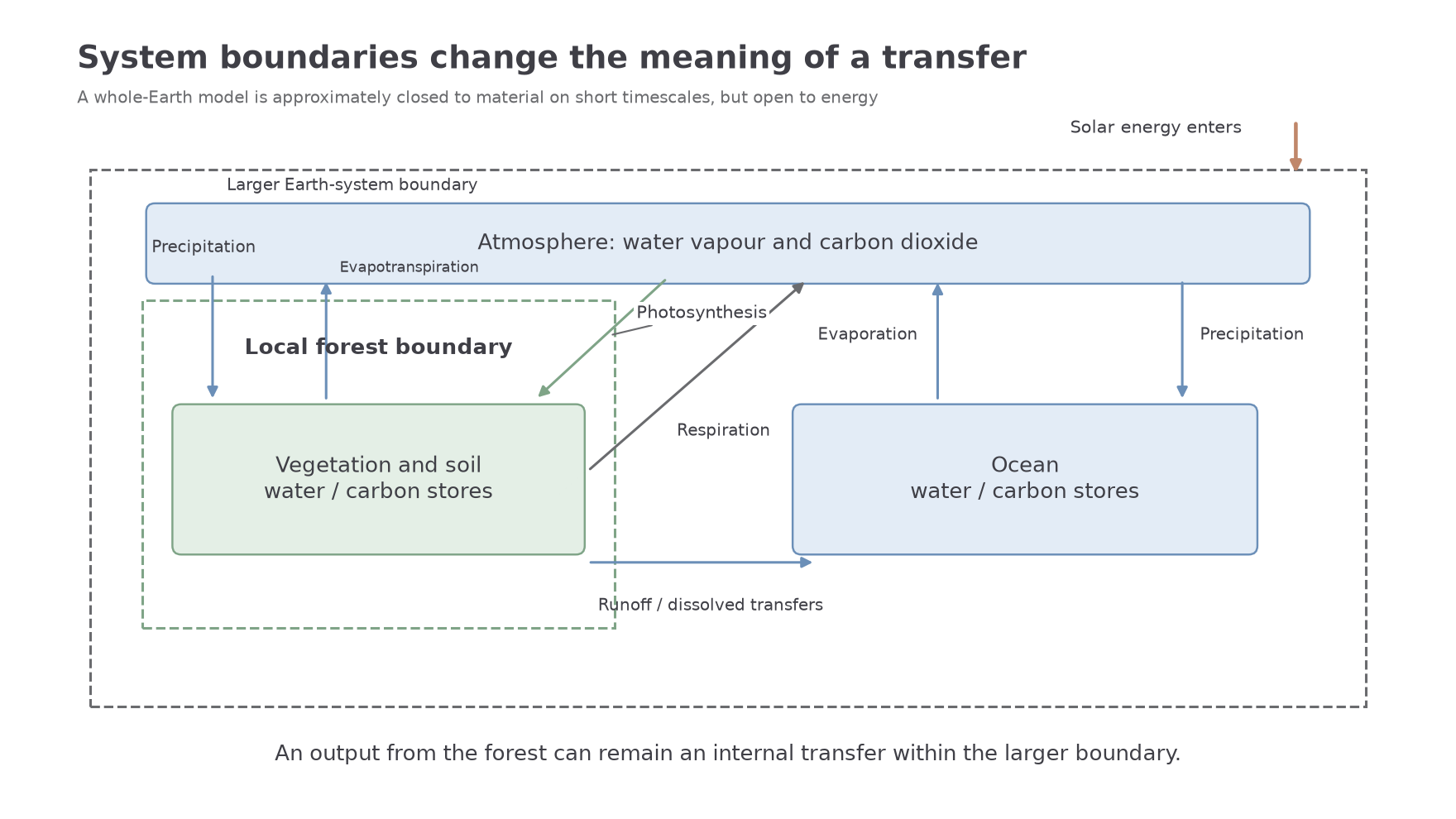
A cycle need not move at a constant rate or return each molecule quickly to its starting point. Water in the atmosphere turns over much more rapidly than water deep within an ice sheet; carbon in a leaf moves on a different timescale from carbon in sedimentary rock. Always state the boundary and timescale before calling a system closed or balanced.
Major water stores
Most of Earth's water is saline, and most freshwater is held outside readily accessible rivers and lakes.
The USGS distribution table, based on Shiklomanov's 1993 reference estimate, provides the following rounded volumes. These are reference estimates of global distribution, not a live inventory for 2026; rounding and classifications affect totals.
| Store | Approximate volume, cubic kilometres | Interpretation |
|---|---|---|
| Oceans, seas and bays | 1,338,000,000 | About 96.5% of total water; mainly saline |
| Ice caps, glaciers and permanent snow | 24,064,000 | About 68.7% of freshwater, but only about 1.74% of total water |
| Groundwater, fresh and saline combined | 23,400,000 | Water in saturated pores and fractures; freshwater part about 10,530,000 |
| Ground ice and permafrost | 300,000 | Frozen ground-associated water; separate from the ice-cap category |
| Lakes, fresh and saline combined | 176,400 | Inland surface stores with contrasting salinities |
| Soil moisture | 16,500 | Water in the unsaturated soil zone, available to roots to differing degrees |
| Atmosphere | 12,900 | Vapour, droplets and ice; small stock with rapid turnover |
| Rivers | 2,120 | Very small instantaneous stock despite important continuing flow |
| Biological water | 1,120 | Water in living organisms, including vegetation |
The denominator matters. Saying that about 69% of freshwater is in ice does not mean 69% of all water is frozen. Similarly, all groundwater is not fresh. A small river store can support a substantial annual flux because it is repeatedly replenished; volume held at an instant and annual volume passing a point answer different questions.
Converting water volumes
Convert the volume by cubing the length conversion. Multiplying cubic kilometres by 1000 instead of one billion confuses length and volume.
Worked volume and share
An artificial lake holds of water within a regional total of . First convert its volume using the cubic multiplier. Then divide matching units to find its share:
The percentage describes that region, with its stated denominator.
Worked freshwater storage comparison
A groundwater store contains within of freshwater. Convert the stock, then find the proportion:
The same groundwater volume would have a smaller percentage if saline water were added to the denominator. A store's volume and its percentage answer different questions.
Major carbon stores
Carbon storage must be compared using the mass of carbon itself and an explicit reference date or baseline.
A gigatonne of carbon, , equals one billion tonnes of carbon, or ; it is also . A tonne of carbon dioxide contains carbon and oxygen, so it is not a tonne of carbon. To convert carbon to carbon dioxide mass, multiply by , the molecular-mass ratio.
The IPCC's 2021 carbon-cycle assessment, Figure 5.12, uses approximate pre-industrial reference stocks with subsequent human-caused changes shown separately. Its scale comparison includes about in vegetation, in soils outside the permafrost region and in permafrost-region stores. Intermediate and deep seawater contain about , far more than vegetation, mainly as dissolved inorganic carbon. The schematic atmospheric baseline is , with a cumulative increase of about by 2019. Do not present any of these baseline stocks as a direct 2026 measurement or assume the categories overlap in the same way in another inventory.
Rocks and geological sediments contain a much larger carbon stock than these rapidly exchanging reservoirs, but exchange much of it slowly. Fossil fuels are a distinct geological store tapped by people. Lakes, rivers and groundwater hold dissolved inorganic and organic carbon and transfer it between soils, oceans and atmosphere. They are smaller global stores but can have substantial local fluxes. Ice is not a carbon reservoir comparable in size to the ocean: important cryosphere-linked carbon is principally in frozen soils and associated organic material, with smaller quantities in trapped gases or dissolved material. Do not substitute the huge volume of frozen water for a huge mass of carbon within the ice itself.
Store-change mass balance
All inputs and outputs must refer to the same boundary and interval. Stocks use ; annual fluxes use . Multiply a constant annual rate by elapsed years before combining it with a stock.
Worked soil budget and carbon conversion
A soil store initially holds , receives 8 tonnes C and loses 6 tonnes C over a year. Calculate the balance and final stock:
The extra carbon's carbon-dioxide mass equivalent is:
The equivalent includes oxygen mass; it does not mean the soil contains 7.33 tonnes of extra carbon.
Worked stock change over several years
A wetland initially holds , with constant annual inputs of 15 and outputs of 18 tonnes C for three years. First find the annual balance, then multiply by time:
The lost carbon has a carbon-dioxide equivalent of:
Large opposing fluxes can coexist with a small net change. A sink gains carbon over the stated interval; a source loses it. Either term depends on the assessed boundary and period.