1.1.2 - Glacial deposits and contrasting landscapes

Moraines and erratics

A glacier deposits material when debris is released, lodged against the bed or accumulated at a margin. Directly deposited glacial sediment, usually called till, commonly contains a poorly sorted mixture of particle sizes. Meltwater can later remove fine material and sort the remaining deposit, so a ridge's present sediment may record more than one process.

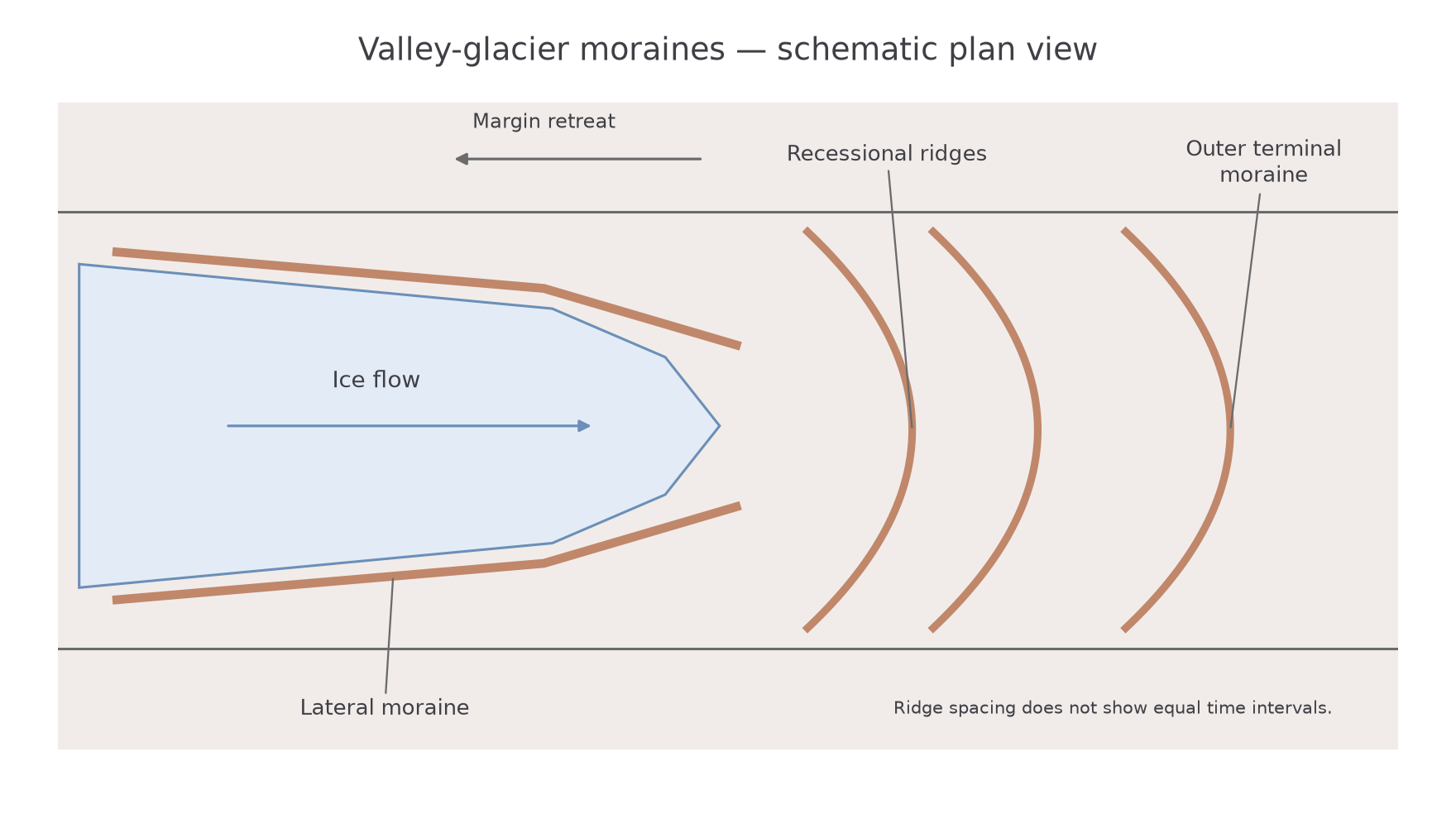
A lateral moraine forms along the side of a glacier from debris supplied by valley walls and transported near the ice margin. Melting and downwasting can leave it as a ridge above a later, smaller glacier or an ice-free valley. Its position can therefore help reconstruct an earlier ice surface, although later slope movement may modify it.

A terminal moraine marks the outermost margin reached during a particular advance or glacial phase. Debris accumulates where supply and release are concentrated near the front; pushing and deformation can also contribute. A temporarily stable front can build a ridge even while individual ice particles continue flowing into it. It is the margin position that is stable, not the whole glacier.

Recessional moraines form at pauses or small readvances during a broader retreat, leaving ridges within the outer limit. A sequence can indicate changing margin positions, but each ridge need not represent an equal time interval. Subsequent rivers can breach and rework them.

[DIAGRAM: asset_name: Moraines and a retreating valley glacier; asset_slug: p11-moraine-plan; caption: Moraine positions record former ice margins while the ice itself continues to flow; description: A schematic valley plan shows present ice upstream, lateral moraine ridges along the sides, recessional ridges beyond the current margin and an outer terminal moraine. Downslope flow arrows and a separate up-valley margin-retreat arrow distinguish ice motion from retreat. No ridge spacing represents elapsed time.]

An erratic is a transported rock fragment whose lithology differs from the bedrock on which it rests. Ice can carry a large block embedded in or supported by it, then deposit it as melting occurs. Matching its rock type to a source helps reconstruct transport, particularly when combined with other directional evidence. An unusual boulder alone is insufficient if several possible sources exist or later processes have moved it.

Drumlins and till sheets

Till can form both broad sheets and streamlined hills beneath ice, depending on sediment supply, bed conditions and the way moving ice deforms or removes material. These forms cannot be explained solely by debris falling from a stationary melting front.

A till sheet is a widespread deposit of poorly sorted glacial sediment. Material can be released from melting ice, pressed or lodged beneath moving ice, or incorporated into a deforming bed layer. A sheet can partly blanket earlier topography, with thickness varying around bedrock obstacles and flow paths. Its broad extent records a distributed depositional system rather than one narrow ice-margin position.

A drumlin is an elongated, streamlined hill, commonly made largely of till, sometimes with a bedrock core. Its long axis is usually aligned with former ice flow. A relatively steep, blunt stoss end and a more tapered lee end can provide a directional clue, especially where many drumlins form a coherent swarm. Individual shapes vary, so material and regional evidence should confirm the interpretation.

Drumlin formation remains an area of research. Plausible mechanisms include deformation and accumulation of sediment beneath moving ice, erosion of pre-existing deposits, and combinations in which erosion and deposition operate at different locations. Basal water pressure and the strength of sediment can influence these processes. Presenting every drumlin as a simple pile dropped behind one obstruction would claim more certainty than the evidence supports.

The contrast with a roche moutonnée is useful. A drumlin is commonly a sediment landform streamlined beneath the ice, whereas a roche moutonnée is an eroded bedrock mound with a smooth stoss and quarried lee. Similar elongation does not make their materials or formation identical. Mapping a group, inspecting sediments and comparing associated striations or erratics makes the reconstruction stronger.

The Lake District valley-glacier landscape

The Lake District in north-west England is a landscape shaped by valley glaciers. Borrowdale and Langdale lie within a central mountain massif whose valleys and lakes form a connected glacial assemblage. Today it is a relict glaciated landscape: rivers, weathering, slope processes and people continue modifying forms produced under earlier ice.

The National Park's geological account identifies resistant volcanic rocks in the central high fells alongside older sedimentary rocks, faults and joints. It also records the broad valleys and sharp ridges left by glaciation. Lake District National Park geology and geomorphology, checked 14 October 2026. Rock strength influences the survival of crags and ridges, while fractures provide routes for quarrying and weathering. The explanation therefore combines lithology and structure rather than assuming resistance prevents erosion entirely.

During glacial conditions, altitude, sheltered hollows and snow accumulation supported corrie and valley ice. Ice moving out of upland hollows joined the valley system, linking corries and ridges with the main troughs. Thicker moving ice could widen and deepen those troughs; differences in erosion left bedrock steps and basins. After retreat, retained water occupied some basins while sediment partly filled others. The National Park's special-qualities account, checked 14 October 2026, describes its radiating glaciated valleys, lakes and continuing geomorphic activity.

The deposits belong to the same system. Debris from valley walls could travel along the ice margins and form lateral accumulations, while changing fronts left moraine and till deposits. Later streams cut through or redistributed that material. A lake, a moraine and a downstream sediment bed are therefore not unrelated features: they can represent linked stages of erosion, storage and reworking.

The current landscape must be read in its historical setting. Present rainfall can cause rockfall or sediment transport, but present valley streams did not necessarily excavate the whole broad glacial trough. Equally, a landform produced by ice is not frozen in its original shape. The case links inherited glacial geometry with ongoing transfers through slopes, lakes and rivers.

A dated example of those continuing transfers is Swindale Beck's 2016 restoration within the managed eastern Lake District landscape. Natural England, the Environment Agency, RSPB and United Utilities restored bends and removed raised banks from an active river corridor. This changed modern flow and deposition within an inherited glaciated valley; it did not create a new glacial trough. Natural England, 13 October 2016.

The west Greenland ice-sheet margin

The Kangerlussuaq–Watson River sector of west Greenland provides the contrasting ice-sheet case beyond the UK. Unlike the present Lake District, this landscape contains an active ice-sheet margin, with outlet ice, exposed bedrock, moraines and a proglacial river system connected to the ocean.

High-latitude conditions limit melt for much of the year, while summer energy inputs generate substantial runoff near the margin. Ice supplied from the interior moves towards lower surface elevations and is affected by bed topography and basal conditions. Crystalline rocks and their fractures influence erosion, but the location and intensity of erosion also depend on where ice slides and meltwater is routed. GEUS's account of the land around the Greenland ice sheet, checked 14 October 2026, explains the geological and erosional setting.

Sediment released beneath or at the margin enters temporary stores, moraines and meltwater channels. The Watson River carries material through the proglacial landscape towards Kangerlussuaq Fjord. Its bars, floodplain and downstream depositional areas respond to water and sediment supplied from upstream, while the proglacial stores can themselves be eroded during floods.

Hasholt and colleagues' study of 2006–2016 estimated mean annual sediment transport of approximately $17.5$ million tonnes through the studied river system, with large differences between years. It identified the proglacial area as a possible net sediment source during high floods. Original research hosted by GEUS. The dated result illustrates a connected ice–river–fjord system; it is not a permanent annual value or proof that all transported sediment was freshly eroded beneath the ice that year.

This case also shows why an ice sheet cannot be treated as one uniform landscape. Thick interior ice, a moving margin and a sediment-rich proglacial channel have different processes and timescales. Greenland's active ice supply contrasts with the Lake District, where later rivers rework sediment inherited from former glaciers.

Glacial change and landscape evidence

A glaciated landscape changes on several timescales, and evidence must match the process being explained. Rockfall may transfer a block in seconds after slow fracture growth. Seasonal melt changes water discharge and sediment transport at an active Greenland margin. Over many glacial cycles, erosion deepens troughs and basins; the Lake District preserves the resulting forms after the ice has disappeared.

In Greenland, a flood can rearrange bars rapidly while the wider ice-sheet margin follows a different trend. Research on the 2010 and 2012 summers compared meteorology, melt, firn and discharge in the Kangerlussuaq sector, showing the value of connecting climatic forcing with measured runoff. Mikkelsen and colleagues' 2016 study, GEUS. In the Lake District today, seasonal river transport reworks inherited glacial sediment; it is not seasonal glacial deposition by a modern local glacier.

Observation begins with what is visible. A ridge can be mapped, its sediment inspected and its relationship to a former ice margin assessed. An interpretation as a moraine should be supported by shape, material and neighbouring evidence. GIS can compare landform alignments, erratic source areas and dated glacier margins, using a common coordinate system and stated positional uncertainty.

Field measurements require a consistent method. A sediment sample might record clast size and shape using a defined transect and selection rule. Choosing only large, easy-to-see clasts biases the distribution. Repeated stream measurements should record location and time because discharge and sediment concentration vary. A photograph alone cannot establish sediment volume or a long-term erosion rate.

Suspended-load rate is discharge multiplied by suspended concentration. A budget then compares all relevant inputs and outputs to find storage change. The following two surveys show the calculations in steps, keeping rate units separate from an interval total.

Worked example — a proglacial survey and sediment loss

Illustrative dataset: five load readings are 5, 6, 6, 8 and 10 kilograms per second. At another measurement, discharge is $16\,\mathrm{m^{3}\,s^{-1}}$ and suspended concentration is $0.35\,\mathrm{kg\,m^{-3}}$. The monitored reach receives 860 tonnes and exports 1,040 tonnes over a season.

The reach loses 180 tonnes from storage. The instantaneous rate of 5.6 kilograms per second is not the seasonal total. If that rate were maintained for a whole day, the estimated export would be $5.6\times86400=483840\,\mathrm{kg}=483.84$ tonnes. Actual daily export needs readings through changing flow conditions.

Worked example — a contrasting survey and sediment gain

Illustrative dataset: a different reach has ordered load readings of 1, 2, 4, 5 and 8 kilograms per second. A separate discharge measurement is $24\,\mathrm{m^{3}\,s^{-1}}$, with suspended concentration $0.15\,\mathrm{kg\,m^{-3}}$. Seasonal inputs are 1,360 tonnes and outputs 980 tonnes.

The second survey has a lower mean but a larger range, so its readings are more spread out on that measure. Its positive storage balance means a net gain of 380 tonnes, although individual channel sections may still erode. Maintaining the measured instantaneous rate for a day would give $3.6\times86400=311040\,\mathrm{kg}=311.04$ tonnes; this is an assumption-based estimate, not an observed daily total. Both suspended-load estimates omit bedload. Unmeasured components, survey uncertainty and changing boundaries can leave a budget residual.

Plotting paired discharge and load readings on a scatter graph can show an association. Sediment availability and previous floods may also influence that pattern, so the graph alone cannot establish one cause.