4.1(c)–(e); 1.1.1–1.1.3 5; 1.2 5; 2.1 6 - Geographical charts, rates and budgets
Geographical representations and calculations reveal patterns only when their scales, units and boundaries are understood. This lesson develops 4.1 information skills and the topic-specific skills in landscape systems, life support and place through chart selection, climate graphs, rates and system budgets.
Choosing charts for geographical variables
Choose a representation by the question and data structure. A line graph can show change through ordered time, while a bar chart compares separate categories. A scatter graph preserves paired measurements and reveals association. A histogram represents a continuous frequency distribution; when class widths differ, the bar area rather than its height must represent frequency, using frequency density. Joining unrelated categories with a line can suggest a continuous sequence that does not exist.
A geographical map answers a spatial question but does not automatically communicate precise quantities well. Proportional symbols can show totals at locations, but symbol area must be proportional to value: doubling a circle's radius quadruples its area. Choropleth shading generally suits rates, percentages or densities over areas. Shading total population can emphasise large administrative areas rather than population concentration. Class boundaries can make similar values appear different or obscure an important threshold, so state the classification.
An illustrative comparison of places might combine a map of service access with a distribution of journey times and selected resident accounts. The map reveals location, the distribution reveals variation, and the accounts explain experience. Each contributes something different; presenting the same ward mean in three colours does not create three independent sources of evidence.
Critique provenance, dates, denominators, scale and missing categories. A change from 10 to 15 cases is a 50% increase, but remains only five additional cases. A truncated vertical axis can amplify the visible difference. Changing ward boundaries can create apparent change without any household moving. Area-level patterns also cannot be automatically assigned to every resident. Explain how a representational choice changes the inference, rather than calling every graph with an imperfect scale “biased” without a reason.
Worked choice and justification
Illustrative resource: annual discharge is measured at one river gauge for 20 consecutive years. A line graph preserves the order and shows fluctuations and trend, with year on the horizontal axis and annual discharge depth on the vertical. A pie chart would divide a whole but would obscure the sequence. By contrast, counts in three unordered land-use categories suit separate bars: joining them would imply a continuous progression between unlike categories. The justification names the data structure and the feature the display reveals.
Worked evaluation of a resource graph
Illustrative graph: two neighbourhood deprivation rates are 10% and 15%, but the vertical axis begins at 9% and the bars have unequal widths. The truncated axis makes a five-percentage-point difference look visually large; clear numerical labels and a disclosed scale help the reader recover its size. Unequal bar widths change apparent area without representing different denominators. Equal-width bars on a clearly labelled percentage axis would improve comparison. A further limit remains: area averages can hide differences within each neighbourhood. This evaluates the actual choices and their consequences.
Worked unequal-width histogram classes
A class spanning 0–10 minutes contains 12 journeys; a 10–30 minute class contains 20. Divide frequency by width so bar area represents frequency:
A separate slope sample has 15 observations in 0–5 degrees and 18 in 5–15 degrees:
The taller bar need not contain more cases when its interval is narrower.
Reading climate graphs
A climate graph commonly combines monthly precipitation bars with a monthly mean-temperature line. They share a time axis but use different vertical axes and units. Read each series against its own scale; a line crossing a bar does not indicate that temperature equals rainfall. A climate graph normally summarises a period's typical conditions, so identify the averaging period rather than treating it as a record of one day's weather.
For an original illustrative location, the monthly values are:
| Month | Jan | Feb | Mar | Apr | May | Jun | Jul | Aug | Sep | Oct | Nov | Dec |
|---|---|---|---|---|---|---|---|---|---|---|---|---|
| Precipitation (mm) | 10 | 12 | 18 | 30 | 50 | 70 | 80 | 70 | 45 | 25 | 15 | 10 |
| Mean temperature (°C) | 5 | 6 | 8 | 11 | 15 | 18 | 20 | 20 | 17 | 13 | 9 | 6 |
Worked annual climate summaries
Sum the twelve precipitation totals, subtract temperature extremes and average the twelve means:
A day-weighted temperature mean can differ because month lengths differ. July and August are warmest, while precipitation peaks in July: this pattern has a wetter warm season.
[DIAGRAM: asset_name: Reading temperature and precipitation on separate scales; asset_slug: h481_s08_climate; caption: Monthly precipitation bars and mean-temperature line use distinct units and vertical axes.; description: An exact illustrative twelve-month climate graph uses precipitation values 10,12,18,30,50,70,80,70,45,25,15,10 millimetres and temperature values 5,6,8,11,15,18,20,20,17,13,9,6 degrees Celsius. Rainfall uses the left axis and temperature the right.]
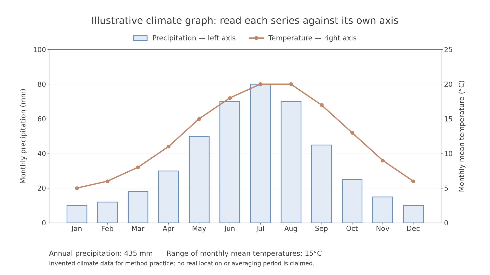
Link the seasonal pattern to processes carefully. Warmer conditions can increase potential evapotranspiration, while rainfall timing affects soil-water recharge. Yet monthly precipitation alone cannot establish a water surplus: evapotranspiration, storage change and runoff also matter. A monthly mean conceals extremes, rainy-day frequency and individual storms. Nor can a climate graph alone explain whether a pattern is caused by altitude, latitude or circulation; location and further atmospheric evidence are needed.
Worked seasonal summaries
A separate cool-season station records three monthly rainfall totals of 42, 58 and 65 millimetres and mean temperatures of 3, 1 and −2°C. Calculate:
Temperature range uses the highest minus the lowest, including the negative sign. These averages indicate seasonal conditions rather than individual storm severity.
Continue this lesson.
You’re previewing NovaLearn without an account. Create a free account to read the rest.
Create free account