H460/03 - Inflation, shocks and distribution

Connected energy markets

An imported input becoming more expensive can shift domestic supply to the left even when demand is unchanged. Suppose an illustrative international gas disruption raises the price paid by bakeries. At each bread price, producing bread is less profitable, so firms supply less. With unchanged bread demand, equilibrium bread price rises and quantity falls. This is a shift of supply followed by a movement along demand, rather than a change in the demand curve caused by the bread price itself.

The size of the price and quantity responses depends on elasticity and time. If consumers cannot easily reduce essential purchases, demand is price inelastic and more of the shock may appear in prices. Bread supply can become more responsive if firms replace equipment or suppliers, but installing these alternatives takes time. Firms do not necessarily pass through every penny: competition, contracts and profit margins affect pricing.

The change spreads to related markets. Consumers may switch towards substitutes for expensive bread. A restaurant using gas and bread faces higher costs from both markets, reducing its supply. Households spending more on essentials have less purchasing power for other goods, reducing demand for discretionary services. The net result in a related market depends on whether substitution, input costs or the income squeeze dominates; identify the relevant relationship rather than saying all demand rises or falls.

Supply shocks and equilibrium

A widespread input-cost increase can reduce short-run aggregate supply, SRAS, rather than merely affecting one product. At any general price level, firms can profitably produce less real output. In an AD–AS model with AD initially unchanged, SRAS shifts left/up: the equilibrium price level rises and real output falls. Reduced output can weaken labour demand, although the employment response depends on firms' hours, productivity and adjustment decisions.

[DIAGRAM: asset_slug: themes-shocks-equilibrium; caption: An illustrative supply shock followed by demand restraint; description: Exact AD-AS intersections show E0 at output eight and price six, E1 at output six and price eight after the supply shock, and E2 at output five and price seven after AD falls.]

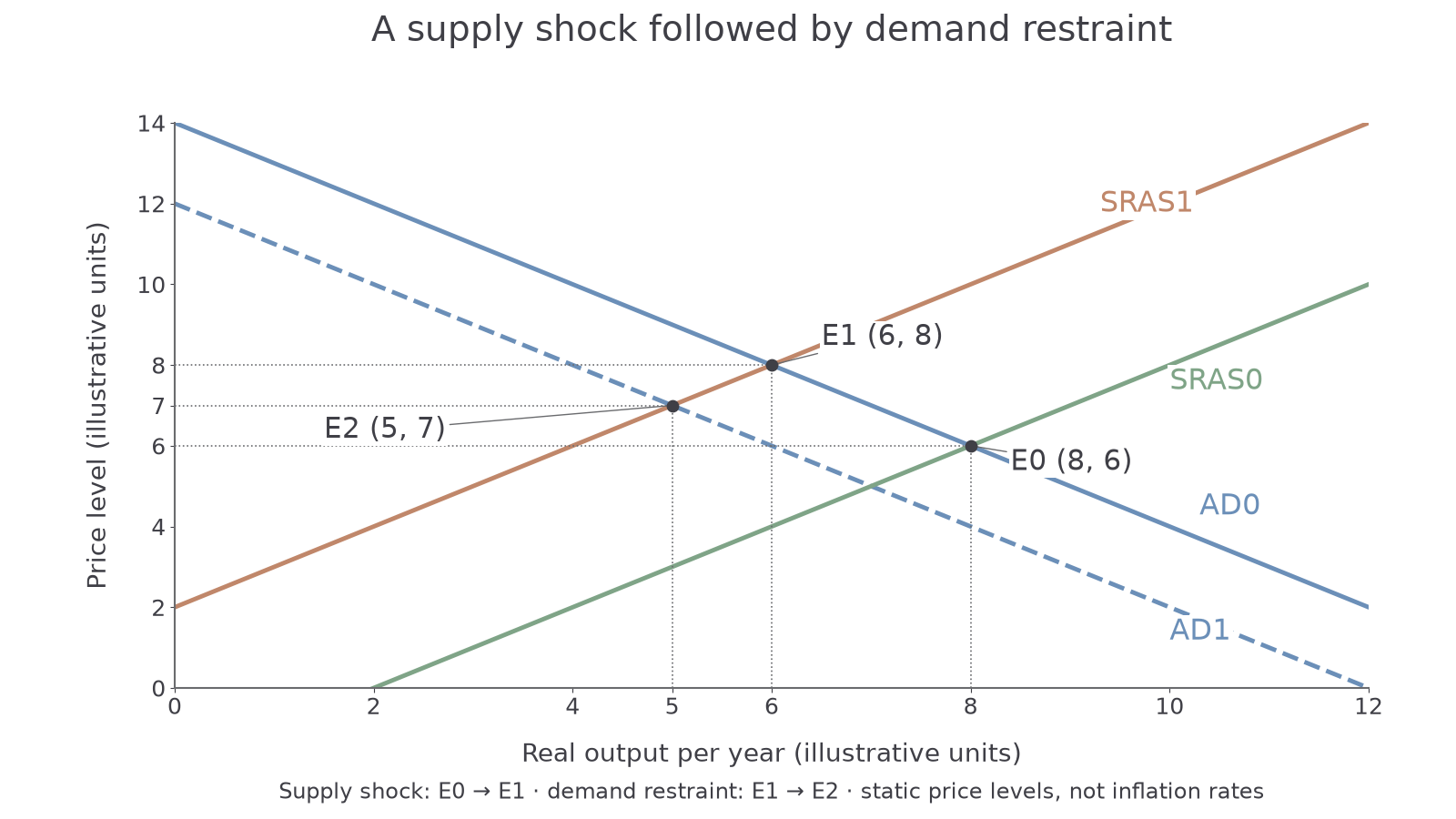
To construct the graph, put the price level on the vertical axis and real output per year on the horizontal axis. Draw downward-sloping AD and upward-sloping SRAS, mark E0, then draw SRAS1 above/left of SRAS0 and mark E1. The numerical scale is illustrative, not measured GDP. It isolates a cost shock by holding AD fixed; confidence or income changes may also shift AD in reality.

Demand restraint then shifts AD left to E2. Relative to E1, both the price level and output are lower, but output is even further below its initial level. Relative to E0, the price level can remain higher. One static diagram compares price levels; an inflation rate requires a change in the price index over time. Repeated cost rises, wage-price responses and expectations determine whether a temporary shock becomes persistent inflation.

If the input price later stops rising, its direct contribution to annual inflation may fade as the higher price enters the comparison base. The original price increase is not thereby reversed. This helps explain disinflation, a falling positive inflation rate, without confusing it with deflation, a fall in the general price level.

Indices and real income

A price index lets us compare purchasing power across dates on a stated common base. In an illustrative economy, the index rises from 100 in Year A to 110 in Year B and 114.4 in Year C. Inflation is 10% from A to B, then 4% from B to C: (114.4 − 110) ÷ 110 × 100. The rate falls by six percentage points, but prices are 14.4% above Year A. The index value 114.4 is not a 114.4% inflation rate.

If a household's nominal income rises from £20,000 in A to £21,000 in B, its 5% money-income increase is smaller than the 10% price rise. Deflate the later income to Year A prices:

The result is £21,000 ÷ 110 × 100 = £19,090.91. Purchasing power falls by approximately 4.55%, not exactly 5%. Subtracting inflation from nominal growth can approximate a small real growth rate; dividing by the price factor gives the exact conversion in this model. Always identify the base and use a price index suitable for the purchasing power being compared.

Constructing an index from a comparable basket costing £250 in the base year and £280 later gives 280 ÷ 250 × 100 = 112. Changes in quality, basket contents and expenditure weights complicate actual measurement. An official average index also need not describe a particular household's consumption pattern.