2.4 - Consumer and producer surplus

Gains from a transaction

Consumer and producer surplus compare the actual transaction price with the reservation prices of the buyer and seller.

Consumer surplus is the difference between what a consumer is willing to pay and what they actually pay. If a buyer would pay up to £9 for a ticket and buys it for £6, consumer surplus is £3. Willingness to pay represents the value of that ticket to that buyer given their circumstances; it is not a cash refund or necessarily a measure of need.

Producer surplus is the difference between what a producer receives and the minimum price at which they are willing to supply. If a seller's minimum acceptable price for the same ticket is £4 and the price is £6, producer surplus is £2. Together, the transaction creates £5 of surplus, the gap between the buyer's £9 valuation and seller's £4 reservation price.

With that one transaction fixed, changing the price from £6 to £7 transfers £1 from consumer surplus to producer surplus: the two become £2 and £3 while their total remains £5. This statement holds the transaction and reservation values unchanged. In a market, a price change can also change the quantity traded and arise because valuations or costs change, so the fixed-transaction example is not a complete market prediction.

Producer surplus is not generally the same as profit. In the standard marginal-cost supply model it is revenue minus variable cost, whereas profit also subtracts fixed cost. A producer can earn surplus from sales while making a loss after the cost of premises is included. Total market surplus also omits unpriced effects on third parties unless those are incorporated explicitly.

Surplus areas on a diagram

Demand and supply curves allow us to add the gains across the units actually traded.

Consumer surplus is the area below demand and above price, up to the quantity purchased. Producer surplus is the area above supply and below price, up to the quantity sold. With straight lines and a common equilibrium, these areas are triangles. The area formula is $\frac12\times\text{base}\times\text{height}$, with quantity as the base and the price difference as height.

[DIAGRAM: asset_slug: h460-foundations-surplus; caption: Consumer and producer surplus are the two areas between demand, supply and the equilibrium price; description: Exact illustrative demand P12 minusQ supply P2 plusQ equilibriumQ5 P7, consumer surplus triangle vertices0 12,0 7,5 7 and producer surplus triangle0 2,0 7,5 7 shaded separately.]

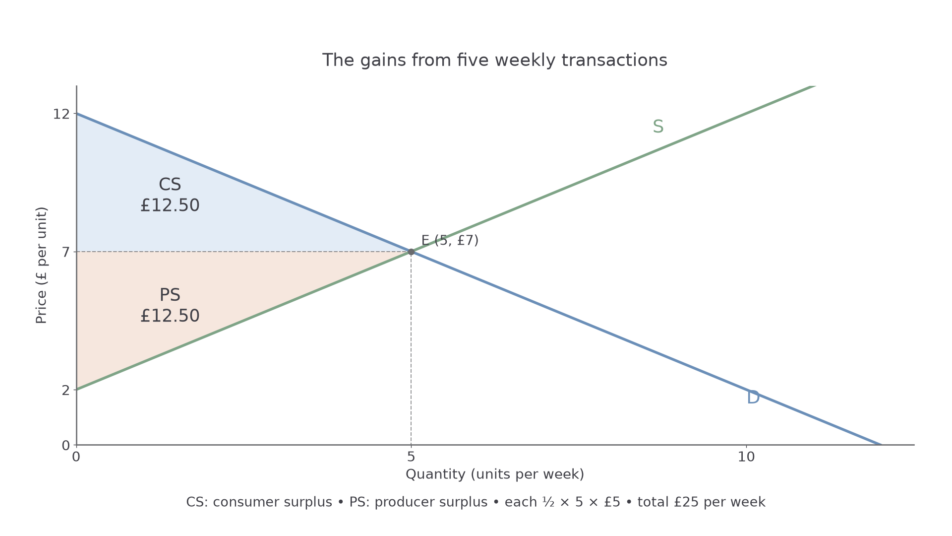
For the illustrative weekly market, five units trade at £7. Both surplus triangles have a quantity base of 5 and a price height of £5.

Consumer surplus is $\frac12\times5\times(12-7)=£12.50$ per week. Producer surplus is $\frac12\times5\times(7-2)=£12.50$ per week. Total surplus is £25, the area between demand and supply up to Q5. Consumer surplus is half of the total here, but equal shares are a feature of these particular lines, not a general law.

The scale matters. If the horizontal axis were thousands of units rather than units, the same numerical triangle would represent thousands of pounds. If the curve is not a straight line or does not start at the axis in the relevant range, the simple triangle formula may not apply. Never calculate the whole price-times-quantity revenue rectangle and call it producer surplus.

To construct the diagram in a notebook, draw correctly labelled demand and supply axes, mark their intersection and the price line, then shade only the relevant areas up to the traded quantity. Surplus lies between reservation values and the actual price, not beneath every curve indiscriminately.

Price effects and their cause

Holding a buyer's valuation unchanged, a lower price increases surplus on that purchase; holding a seller's reservation price unchanged, a higher price increases surplus on that sale.

For a whole market, specify which curves changed. With a fixed demand curve and sufficient supply for the quantity buyers demand, a lower price expands consumer surplus: existing buyers pay less and additional purchases can create extra surplus. With a fixed supply curve and sufficient demand for the quantity offered, a higher price expands producer surplus: existing units receive more and additional worthwhile units can be sold. These are separate comparisons, not a claim that arbitrary demand and supply quantities both trade at a disequilibrium price.

[DIAGRAM: asset_slug: h460-foundations-surplus-changes; caption: Different shifts change surplus as well as price, so a price fall alone does not prove producers lose; description: Exact two panels initial D P12 minusQ S P2 plusQ Q5 P7; demand increase to P14 minusQ Q6 P8, and supply increase to P Q Q6 P6, showing old and new consumer and producer surplus geometry.]

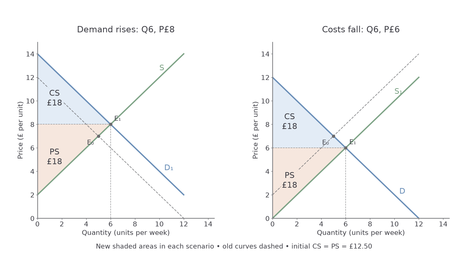
In the demand-shift scenario, valuations change. In the supply-shift scenario, costs change. The two new equilibria cannot be interpreted as changes in price alone.

In the first scenario, demand rises from $P=12-Q$ to $P=14-Q$, with supply unchanged. New equilibrium is Q6, P8. Producer surplus rises to $\frac12\times6\times(8-2)=£18$. Consumer surplus also becomes $\frac12\times6\times(14-8)=£18$: higher willingness to pay and more purchases outweigh the higher price in this example. It is wrong to infer lower consumer surplus merely because price rose.

In the second scenario, supply expands from $P=2+Q$ to $P=Q$, with demand unchanged. Equilibrium is Q6, P6. Consumer surplus becomes $\frac12\times6\times(12-6)=£18$. Producer surplus becomes $\frac12\times6\times(6-0)=£18$. Producers receive less per unit, but their lower reservation prices and larger quantity make surplus rise. Different shift shapes can give different distributions: calculate or inspect the actual areas.

Judging gains and distribution

A surplus comparison should separate a transfer between traders from a change in the total gains and consider the model's limits.

For an unchanged completed transaction, a higher price transfers surplus from the buyer to the seller without changing the valuation-cost gap. When quantity changes, additional mutually beneficial trades can increase total surplus. In the supply-improvement example, total surplus rises from £25 to £36; this is not merely a transfer. A cost reduction changes the real resource cost as well as the market price.

Aggregate gains do not mean that every individual gains. An average consumer-surplus increase can conceal buyers who face an inconvenient product change or cannot access the market. A producer-surplus increase for the industry can coexist with losses for a particular high-cost firm that loses sales. To judge distribution, identify the affected groups instead of treating consumers and producers as two identical individuals.

The diagram assumes the relevant demand and supply relationships represent willingness to pay and marginal opportunity costs adequately. Income differences affect willingness to pay. External harm such as pollution may not enter private supply, so higher private total surplus is not automatically higher social welfare. A distorted or rationed market may also allocate units to buyers other than those with the greatest willingness to pay, altering the predicted area.

For an illustrative technological improvement, lower costs and a larger traded quantity make higher total surplus plausible, and the numerical example shows both groups gaining. The claim becomes weaker if the technology causes unpriced damage or the demand comparison mixes different product quality. A defensible judgement states the source of the change, compares the actual areas and qualifies the welfare conclusion using a relevant limitation.

Quick recap

Consumer surplus lies below demand and above price; producer surplus lies above supply and below price. Calculate with the actual traded quantity and units. Identify the cause of a price change before judging gains, and distinguish transfers, additional gains and effects the private-market model omits.