1.4 - Macroeconomic equilibrium and shocks
An increase in spending can raise output, prices or both, depending on the economy's ability to supply more. Learn to locate macroeconomic equilibrium, trace demand and supply shocks, and compare what Keynesian and neo-classical assumptions imply for employment and the price level.
What the model holds constant
An AD–AS model combines planned expenditure on domestic output with firms' supply decisions at different general price levels.
The vertical axis is the price level, such as an index, and the horizontal axis is real output, such as GDP at constant prices. AD slopes downward for the aggregate mechanisms taught in 1.2; it is not an individual product's demand. In a short-run model, SRAS slopes upwards because some input prices and other costs do not immediately rise with output prices. Higher output prices can then make extra production profitable, although increasingly scarce resources raise marginal costs.
Each curve holds other determinants constant. Moving along SRAS following a price-level change is different from shifting SRAS after a rise in imported input costs. A rise in government purchases shifts AD, rather than causing a movement along it. When describing a shock, change the relevant determinant first and retain the other curve initially; otherwise the drawing cannot isolate the mechanism. Secondary effects can be explained subsequently.
The neo-classical long-run model assumes sufficient adjustment of wages and prices for output to return to sustainable potential, represented by vertical LRAS. The Keynesian model allows deficient spending and sticky prices/wages to sustain unemployment. Its aggregate supply curve is relatively flat with abundant idle resources, becomes steeper as bottlenecks appear, and is vertical at full capacity. These are alternative assumptions about adjustment and spare resources, rather than contradictory claims about one unchanging supply curve. Neither automatically predicts how quickly an actual economy adjusts.
Equilibrium and adjustment
Macroeconomic equilibrium is the combination of real output and price level at which aggregate quantity demanded equals aggregate quantity supplied.
At the AD–SRAS intersection, planned spending matches the value of output supplied in the model. If firms produce more output than buyers demand at a given price level, inventories may accumulate unexpectedly; firms reduce production and possibly prices. If demand exceeds output supplied, inventories can fall and firms raise production or prices. Price/wage stickiness, delivery delays and uncertainty mean this is an adjustment tendency rather than an instantaneous auction.
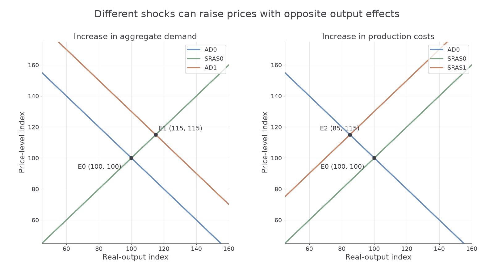
An illustrative equilibrium is E0 at real output 100 and price index 100. The numbers are model indexes, not observed national data. Draw both labelled curves, mark the intersection and use dashed guides to read each coordinate. Compare real output with potential output separately: AD = SRAS at 100 does not prove 100 is full-employment output. Equilibrium means plans match; full employment allows normal frictional/structural unemployment but no demand-deficient spare capacity. The two concepts can differ.
Lower real output will usually require fewer labour hours and can increase cyclical unemployment, holding productivity and working practices constant. It is not a mechanical one-for-one relationship: firms may retain workers, adjust hours or change productivity. A higher price level is a rise in the index; inflation is its rate of increase over time. A single shock that raises the level once need not produce permanently accelerating inflation.
Demand shocks and cost shocks
A spending shock changes AD, whereas a production-cost shock changes SRAS; the distinction explains why prices and output can move in different directions.
Suppose stronger confidence raises consumption and investment at each price level. AD shifts right from AD0 to AD1 with SRAS initially unchanged. The new equilibrium has higher real output and a higher price level. Firms expand production to meet sales, and labour demand may rise. If there is substantial spare capacity, most of the effect may be on output; with widespread bottlenecks, more can be on prices. A fall in confidence reverses the initial direction, lowering output and easing price pressure; sticky prices can mean the adjustment is mostly in quantities initially.
An increase in imported energy costs raises firms' unit costs. At each price level they supply less, shifting SRAS left/up. Real output falls while the price level rises: a negative supply shock can therefore combine weak activity with cost-push inflation. A sustained rise in productivity can lower unit costs and shift SRAS right/down, increasing output while reducing the price level relative to the no-change position.
[DIAGRAM: asset_slug: ocr_h460_demand_cost_shocks; caption: Increased AD raises output and prices; a negative cost shock lowers output while raising prices; description: Exact two-panel AD–SRAS comparison from E0(100,100), with demand expansion E1(115,115) and adverse supply shift E2(85,115).]
Continue this lesson.
You’re previewing NovaLearn without an account. Create a free account to read the rest.
Create free account