1.3 - Opportunity cost and production possibilities

The next-best alternative

Opportunity cost is the value of the next-best alternative forgone when a choice is made.

A trade-off is the sacrifice involved in obtaining more of something else. Opportunity cost identifies the best forgone alternative, rather than adding every rejected option together. If you choose to study instead of taking a paid shift or watching a film, and the shift was your next-best option, its forgone value is the relevant opportunity cost. The film is not an additional cost on top of it.

Money expenditure and opportunity cost can differ. A room already owned by a college has no new purchase price when used for tutoring, but it could have been rented out or used for another class. Conversely, an unrecoverable past payment should not be treated as a new sacrifice caused by today's choice. Compare the benefits and resources that actually change between feasible alternatives.

In an illustrative workshop, the same two hours could make four stools or repair six chairs. Choosing four stools sacrifices six chair repairs, so the opportunity cost is six repairs in total or $6/4=1.5$ repairs per stool. In the reverse direction, one repair costs $4/6=2/3$ of a stool. State the denominator and units: reciprocal costs are not the same number.

The concept applies to households, firms and government. Time spent commuting sacrifices other uses; a firm using a site for storage gives up another use; spending on one public project sacrifices the next-best use of the funds and resources. It makes “free” policies and choices visible as real resource decisions.

Reading a PPC

A production possibility curve shows the maximum feasible combinations of two outputs with given resources and technology.

The model assumes a stated period, resources and technology, and reduces an economy's many outputs to two categories. Points on the PPC are productively efficient: more of one output requires less of the other. Points inside are feasible but productively inefficient, for example because some labour is unemployed or resources are poorly organised. Points outside are unattainable with the current productive capacity; they may become feasible after a capacity increase.

[DIAGRAM: asset_slug: h460-foundations-ppc; caption: A bowed PPC separates efficient, inefficient and currently unattainable production; description: Exact illustrative PPC with equipment units per week on the horizontal axis and food units per week on the vertical axis, Y equals100 minusX squared, frontier points A0 100 B4 84 C8 36 D10 0, inside I4 50 and outside U8 80.]

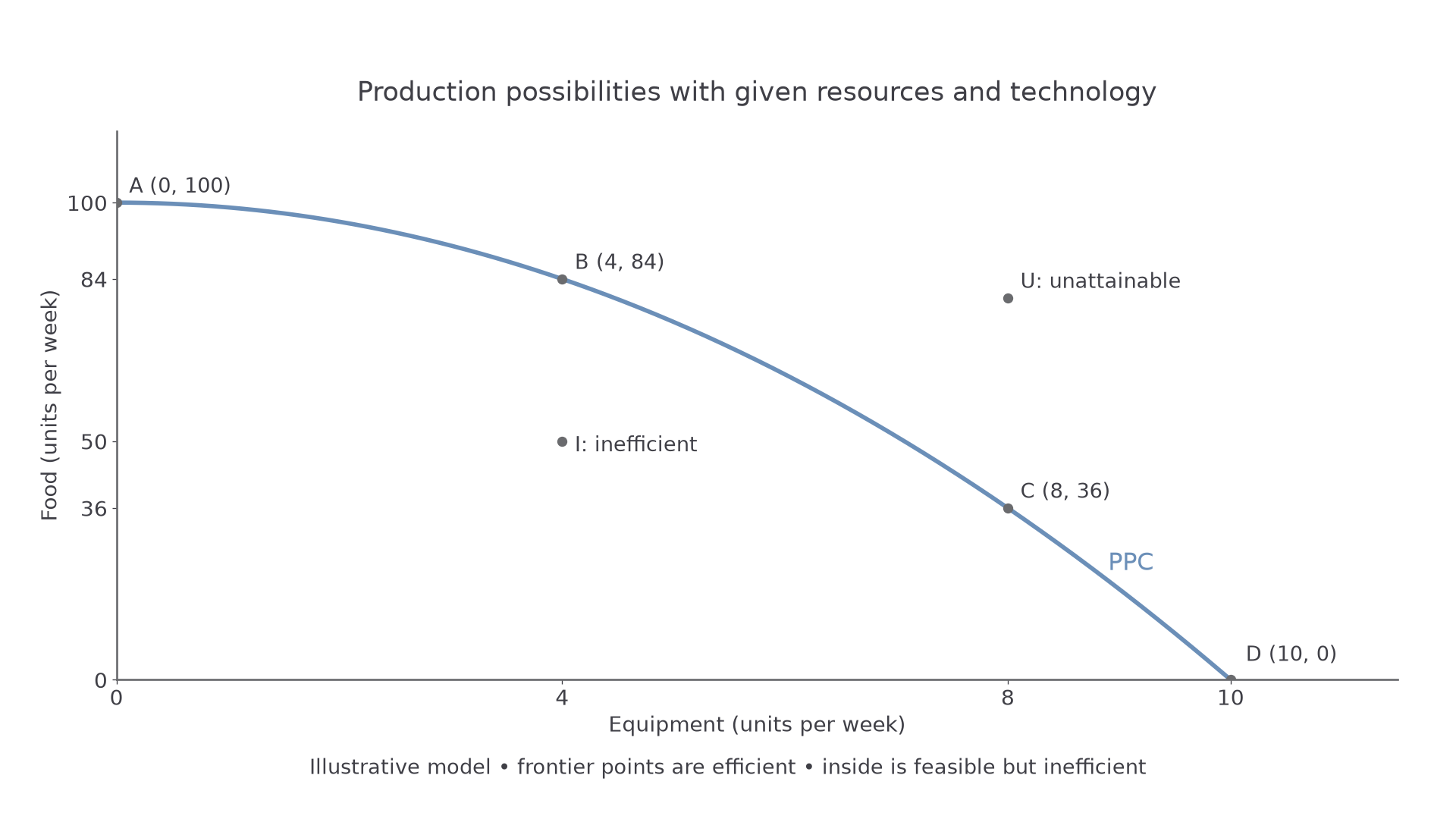
Illustrative weekly production possibilities: food $Y=100-X^2$, where $X$ is equipment output from 0 to 10. The curve describes a model, not observed national data.

To construct this PPC in a notebook, label both output axes and the period, plot the combinations (0,100), (4,84), (8,36) and (10,0), and join them with the bowed frontier. Mark I at (4,50) inside and U at (8,80) outside. A curve drawn beyond the stated equipment maximum would assert production the schedule does not permit.

At B, all resources are used efficiently, but that does not establish allocative efficiency. Society may prefer a different efficient combination. The PPC alone does not reveal preferences or which people receive the food and equipment. Efficiency on the frontier is therefore a statement about production possibilities, not a judgement that the chosen distribution is fair.

Movements and opportunity cost

A movement along an unchanged PPC reallocates existing productive capacity between the two outputs.

In the plotted example, moving from B (4 equipment, 84 food) to C (8 equipment, 36 food) gains four equipment units and sacrifices 48 food units. The average opportunity cost of each additional equipment unit over that interval is $48/4=12$ food units. Equipment output rises by $(8-4)/4\times100=100\%$, while food output falls by $(36-84)/84\times100\approx-57.1\%$. The percentages use different initial output bases, so they need not match.

Moving from A to B sacrifices only 16 food units for four equipment units: four food units per equipment unit. The bowed frontier represents increasing opportunity cost. Resources are not equally suited to each activity. As equipment production expands, it draws in resources increasingly valuable in food production, so the next equipment unit requires a larger sacrifice. A straight-line PPC instead assumes constant opportunity cost, such as resources equally adaptable at a fixed conversion rate.

Moving from I (4,50) to B (4,84) increases food without reducing equipment. This is better use of existing capacity, not an outward shift of the frontier. Moving from B to C is a change in output mix, not proof that the economy's capacity has increased. A fall in one output alone cannot distinguish a reallocation, unused capacity or a contraction of capacity; the whole model matters.

Capacity changes and useful choices

A shift of the PPC changes what can be produced, rather than merely changing the chosen combination.

More usable resources, better skills or technological improvement can move the frontier outwards. A new food-growing technique may expand only food capacity, causing the PPC to pivot; technology benefiting both activities can expand both intercepts. Destruction of factories, loss of usable land or a sustained fall in available labour can shift it inwards. Temporary idle factories are normally represented by production inside the existing frontier, not by a smaller frontier.

[DIAGRAM: asset_slug: h460-foundations-ppc-shift; caption: A capacity expansion shifts the PPC outwards, while recovery from idle resources moves production towards the old frontier; description: Exact old PPC Y100 minusX squared and new PPC Y120 times1 minus X over12 squared, labelled PPC0 PPC1, showing movement I4 50 to B4 84 within unchanged capacity.]

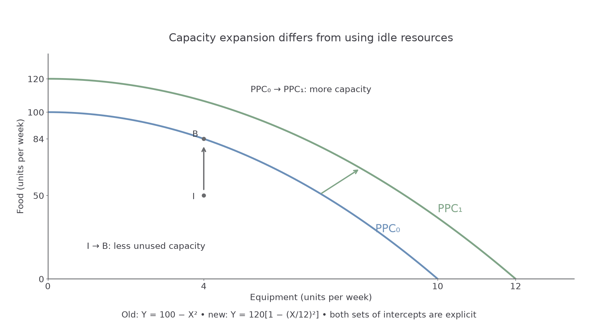
The new illustrative frontier has food intercept 120 and equipment intercept 12. Its position represents additional capacity, independently of where actual production occurs.

The food intercept rises from 100 to 120: $(120-100)/100\times100=20\%$. A point's two output coordinates may change by different percentages, so one intercept change does not establish a unique overall growth rate for the whole economy. Real economies also have many outputs, changing quality and price weights that this two-good picture omits.

Opportunity cost improves decisions by comparing gains with the best forgone use. If a council uses a site for a sports centre, the benefits must be compared with the best feasible alternative use of that site and funding. An outward shift makes more combinations possible but does not choose between them. Nor does a diagram quantify satisfaction, environmental damage or fairness without further evidence.

For investment, sacrificing some current consumption to produce equipment may expand future capacity. That is a possible causal link, not a guarantee: the equipment must be useful and maintained, and the current sacrifice matters to households. Opportunity cost is particularly useful where market prices hide donated time, owned land or alternatives with no direct cash payment. Its practical limitation is identifying and valuing the true next-best alternative, especially under uncertainty.

Quick recap

Opportunity cost values the next-best alternative forgone. Movements along a PPC change the output mix, movements towards it reduce inefficiency and shifts change capacity. Read output units and bases carefully; the frontier does not by itself settle social preferences or fairness.