4.2 - Monopoly, output and efficiency

Monopoly power and entry barriers

A pure monopoly is the only supplier in a defined market, while monopoly power more generally is an ability to influence price.

The market definition matters. A supplier may be alone in a narrow local market yet face substitutes in a wider one. A monopolist faces market demand rather than the perfectly elastic demand of a small price-taker. It can choose a price–quantity combination on that demand curve, not both independently: charging a higher price usually reduces purchases.

Barriers to entry protect this position. Legal rights such as patents or exclusive licences can restrict rivals; control of a necessary resource or distribution network can prevent access; economies of scale may make entry at a small scale costly. Brand loyalty, switching costs and network effects can also weaken entrants. Some barriers reflect useful innovation or infrastructure; others protect an incumbent without such benefits.

An illustrative software supplier develops a valuable program. Copyright protects its code, while compatibility with customers' files raises switching costs. These conditions may limit rivalry, but alternatives that perform the same task still constrain demand. Monopoly power is a matter of available substitutes and credible competition, not simply a large business or high revenue.

Entry barriers can sustain supernormal profit in the long run. They do not guarantee it: demand may be too weak or costs too high. A monopolist can earn normal profit or make losses, even while choosing its best available output.

Revenue and the output decision

A single-price monopolist earns less marginal revenue than average revenue because selling more normally requires lowering the price on existing sales.

Its AR curve is demand: TR/Q equals the price paid per unit. With a downward-sloping demand curve, a price cut earns revenue on the additional units but loses revenue on the units already sold. Thus MR lies below AR. For linear demand, MR has the same vertical intercept and twice the downward slope. That geometric rule applies to linear demand, not every curve shape.

An illustrative demand schedule is $P=20-Q$, with Q in thousands of units and price in pounds. At Q=6, P=£14 and TR=£84,000; at Q=7, P=£13 and TR=£91,000. The additional thousand units raise TR by £7,000, much less than the £13,000 earned on them alone, because the previous six thousand sales now earn £1 less each. The discrete revenue change differs from point MR at an endpoint; both show why AR and MR differ.

Profit maximisation uses rising MC=MR. Find that output on the horizontal axis, then move up to AR to read price. MC=MR locates output, not the price charged. Reading price from MR is a common error. A profit-maximising single-price monopolist with positive MC normally operates in the elastic portion of demand, where MR is positive; expanding in the inelastic portion would reduce TR while increasing cost.

[DIAGRAM: asset_slug: h460-monopoly-output; caption: Monopoly output is where MC meets MR; price comes from AR and exceeds MC; description: An exact illustrative cost-consistent diagram with downward AR and MR, MC crossing MR at Qm, the monopoly price on AR, AC below that price and an allocatively efficient benchmark where AR meets MC.]

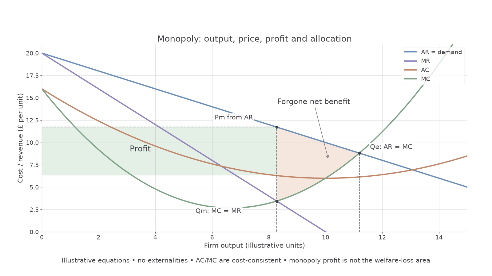
To construct the diagram, label vertical cost/revenue per unit and horizontal output. Draw downward AR, lower MR, and a cost-consistent rising MC intersection with MR. Mark Qm vertically, then mark Pm from AR at Qm. Add AC and read it at Qm to identify profit. MC need not equal AC at Qm: that equality identifies minimum AC, not profit maximisation generally.

Profit and static efficiency

Monopoly profit and efficiency are separate questions, requiring different comparisons in the same diagram.

At Qm in the supplied diagram, Pm>AC, so economic profit is $(Pm-AC)Qm$, the shaded rectangle. Durable barriers can preserve this profit in both short and long run. A lower demand curve or higher AC could remove it without changing the basic decision rule.

For a transparent illustrative calculation, a monopolist sells 6,000 units at £14 with AC £8. TR=£84,000, TC=£48,000 and economic profit=£36,000. Marginal revenue and marginal cost are used to find the chosen output; their difference is not total profit. To find average profit, divide total profit by Q, giving £6 per unit.

In the standard no-externality model, allocative efficiency requires P=MC. The monopolist has P>MR=MC, so some units valued by buyers above their marginal cost are not supplied. The diagram's efficient benchmark Qe is where AR meets MC. The area between AR and MC from Qm to Qe represents lost net benefit under these assumptions. Monopoly profit is partly a transfer from consumers to the producer; it is not itself identical to this welfare loss.