1.2 - Aggregate demand and consumption

Spending on domestic output

Aggregate demand is total planned expenditure on an economy's domestically produced goods and services at each price level, over a stated period.

Consumption buys goods and services for use by households, from food to haircuts. Investment buys capital goods or adds to inventories: a bakery's new oven is investment; purchasing an existing company's shares is a financial transaction, not itself new output. Government expenditure includes purchases such as teachers' services and road construction. A benefit payment is a transfer; it enters AD if its recipient subsequently spends it, rather than being counted as both G and C.

Exports are purchases of domestic output by overseas buyers. Imports are subtracted because imported spending may already appear in C, I or G but does not demand domestic production. Subtracting M is an accounting adjustment, not a claim that importing is harmful.

In an illustrative economy, annual planned C is £600 billion, I is £140 billion, G is £220 billion, X is £180 billion and M is £200 billion. AD is $600+140+220+180-200=£940$ billion. If households spend an extra £10 billion entirely on imports, both C and M rise by £10 billion; direct spending on domestic output is unchanged. Domestic transport or retail services could create an additional domestic effect, but none is assumed in this example.

Why the AD curve slopes down

The AD curve relates the general price level to the quantity of real domestic output demanded, holding other determinants of spending constant.

Its vertical axis is the price level, often represented by a price index. Its horizontal axis is real output, not the quantity of a single product. A lower price level does not simply make households substitute one domestic good for another: that reasoning belongs to an individual market.

Three mechanisms can explain a downward slope. First, a lower price level raises the purchasing power of existing money balances and some fixed nominal assets, encouraging spending: the real balance effect. Second, holding nominal money supply constant in a simple money-market model, fewer nominal balances are needed for a given volume of transactions; lower interest rates can encourage borrowing and spending. This interest-rate explanation assumes a monetary setting in which rates respond in that way. Third, domestic prices falling relative to overseas prices can make exports more competitive and imports less attractive, increasing net exports, with the exchange rate held constant. The size of this effect depends on how trade quantities respond to relative prices.

An economy may therefore demand more real output when its price index falls from 110 to 100. That is an extension of AD, a movement down the same curve. It does not mean that every household spends more or that nominal expenditure must rise: nominal expenditure depends on both prices and quantities.

[DIAGRAM: asset_slug: ocr_h460_ad_movement_shift; caption: A price-level movement along AD and an increase in AD at a fixed price level; description: Two-panel AD graph with real output on the horizontal axis and price index on the vertical axis, showing movement along AD0 and a rightward shift to AD1.]

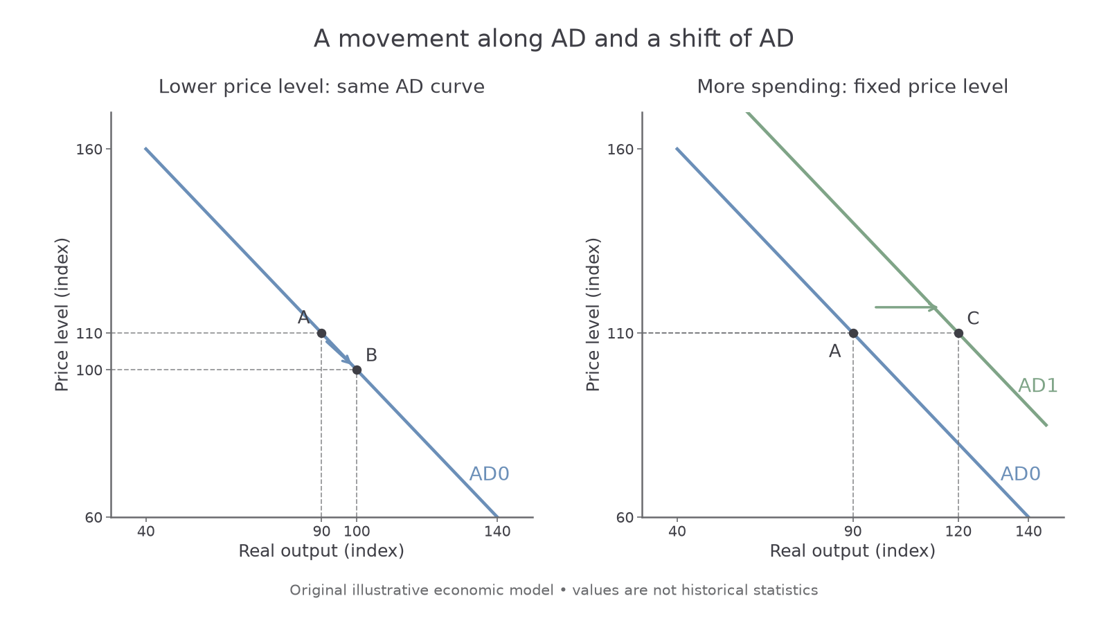
The plotted numbers are illustrative. In the left panel, A to B changes the price level on AD0; in the right panel, A to C changes output demanded at the same price index of 110. These are different explanations even when output demanded rises in both cases.

To sketch the claim in a notebook, put price level on the vertical axis and real output on the horizontal axis, then draw and label a downward-sloping AD curve. Mark two positions on that same curve for a price-level movement. For changed spending at a fixed price level, draw a second labelled curve and compare the output demanded on the two curves along one horizontal price-level line. Reading a supplied graph here does not assess your independently drawn graph.

Changes in planned spending

The AD curve shifts when planned expenditure on domestic output changes at a given price level.

If households become confident that employment will remain secure, they may buy more durable goods now. C rises at each price level, so AD shifts right. If firms expect fewer future sales, they may postpone capital purchases: I falls and AD shifts left. An increase in government purchases or stronger overseas demand for exports can shift AD right; a fall can shift it left. Detailed investment, fiscal and trade mechanisms are developed in their own lessons.

Always identify the initial change. A fall in the general price level, with other determinants constant, causes a movement along AD. A cut in an interest rate set by the central bank can shift AD through consumption and investment even before the price level changes. An appreciation of the currency can reduce net exports at the initial domestic price level, shifting AD left. A rise in one product's price is not automatically a rise in the economy's price level.

Expectations are beliefs about future income, sales, costs or policy. They affect present decisions because purchases and borrowing commit resources over time. News of likely unemployment may reduce consumption before anyone actually loses a job. The resulting fall in firms' sales can weaken investment as well. Expectations can therefore magnify an initial change, but the effect is conditional: households with secure income may respond little, and constrained households may already lack funds to change spending.