2.6 - Price elasticity of demand and revenue
A price rise earns more on each sale but may lose customers. This part of 2.6 teaches how price elasticity of demand measures that response, how it affects revenue, and how a firm can judge whether an estimate is useful. Income elasticity, cross elasticity and price elasticity of supply are taught in the other 2.6 lessons.
Calculating PED
Price elasticity of demand compares the proportional change in quantity demanded with the proportional change in the good's own price.
Elasticity measures responsiveness: how strongly one variable responds to a change in another. Price elasticity of demand (PED) is the percentage change in quantity demanded divided by the percentage change in price, with other influences on demand held constant. Percentages allow comparisons between goods sold in different units and at different prices.
Price elasticity of demand
For a change from an initial value, .
Use the original value as the denominator unless the task specifies another method. Do not divide the change in quantity measured in units by the change in price measured in pounds: that produces a slope measure, not elasticity. PED has no currency or quantity unit.
Distinguish percentage changes from percentage-point changes when the starting variable is itself a percentage. A share rising from 20% to 25% increases by 5 percentage points, but by 25% relative to its initial value. PED uses relative percentage changes in price and quantity, not a subtraction of percentage-point labels.
A worked calculation
In an illustrative market, a museum raises admission from £10 to £11. Weekly quantity demanded falls from 400 to 340 visits. Assume income, tastes, rival prices and other demand conditions are unchanged.
The price change is . The quantity change is . Therefore .
The negative sign shows the opposite directions of change along the ordinary downward-sloping demand curve. The magnitude, 1.5, means a 1% price rise is associated with approximately a 1.5% fall in quantity demanded around the relevant situation. It does not mean quantity falls by 1.5 visits or by £1.50.
Keep the sign in a signed calculation. Economists often discuss the absolute value, , when classifying responsiveness. Thus “PED is −1.5” and “the absolute elasticity is 1.5” convey the same response with different sign conventions.
A fall in price usually gives a positive percentage quantity change and a negative percentage price change, so PED is still negative. Check the direction, denominator and percentage units before deciding that an unexpected answer reveals unusual consumer behaviour.
Interpreting responsiveness
The absolute value of PED tells us whether quantity responds more or less than proportionately to a price change.
| Absolute PED | Description | Meaning |
|---|---|---|
| 0 | Perfectly inelastic | Quantity demanded does not respond to price. |
| Between 0 and 1 | Price inelastic | Quantity changes by a smaller percentage than price. |
| 1 | Unit elastic | Quantity changes by the same percentage as price under the stated calculation. |
| Greater than 1 | Price elastic | Quantity changes by a larger percentage than price. |
| Approaches infinity | Perfectly elastic | Buyers will purchase at the given price but not at any higher price in the model. |
These are response categories, not labels for whether demand is high or low. A firm can sell very many units to customers whose demand is inelastic. Conversely, a small market can have elastic demand.
[DIAGRAM: asset_slug: h460-ped-extremes; caption: Vertical demand has zero PED and horizontal demand is perfectly elastic in the limiting model; description: Two exact illustrative demand plots with price on the vertical axis and weekly quantity on the horizontal axis, showing vertical and horizontal demand.]
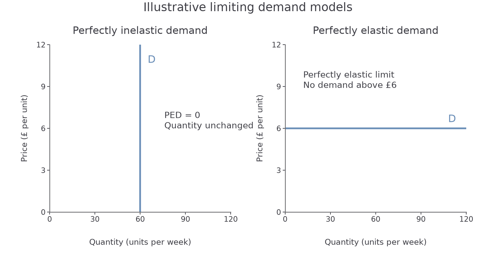
The extreme cases isolate the meaning of responsiveness. They are limiting models rather than a claim that real consumers never change their decisions.
On the vertical curve, quantity stays at 60 units as price changes. On the horizontal curve, a price above £6 loses the demand represented by this model. Do not interpret the horizontal case as buyers being willing to pay any price.
Drawing a demand curve correctly requires price on the vertical axis and quantity demanded on the horizontal axis. Label the curve D, label both variables, and give units when using numerical scales. A movement along D follows a change in the good's own price; a change in income or a rival's price shifts demand and cannot by itself identify own-price PED.
The slope of a curve and its elasticity are related but are not identical. A straight downward-sloping demand curve has constant slope, yet PED varies because the initial price and quantity vary. Visual steepness also depends on the axis scales. Compare two curves' responsiveness only with meaningful common scales and a stated point or price range. The next revenue section shows why one straight line can contain both elastic and inelastic regions.
Why responsiveness differs
Consumers respond to a price rise according to the alternatives they can use and the adjustments they can make.
Availability and closeness of substitutes are central. If one café raises its price while similar cafés nearby do not, consumers can switch easily. Demand for that café may be elastic. If every café raises prices, switching between cafés no longer avoids the increase: demand for the broader category can be less elastic. The market definition therefore matters.
Necessity and habits can limit adjustment. A medicine needed to control a condition may have inelastic demand if there is no effective substitute. A discretionary entertainment purchase can be postponed. This is a reasoned tendency, not a rule that every “necessity” has the same PED: a necessary journey may still have substitutes such as a bus, a train or a different route.
The share of a household's budget affects the incentive to search or economise. A small price increase on an inexpensive occasional purchase may hardly affect the budget. A comparable percentage rise in rent or a major durable can prompt substantial adjustment. Income, preferences and who pays the bill can change that response.
Time often increases responsiveness. Immediately after a fuel price rise, a commuter may have little choice but to drive an existing car. Over time the commuter can arrange a car share, move nearer work, change vehicle or use public transport. Demand is often more elastic in the long run, provided those alternatives actually become feasible.
An explanation should connect the condition to behaviour. “There are substitutes” is only a starting point: close alternatives permit switching, so a given percentage price rise causes a larger percentage reduction in purchases. Similarly, a lack of alternatives constrains switching and tends to reduce the proportional quantity response.
Several factors can pull in different directions. A luxury with a loyal following may face weak substitution; an essential branded product may face close generic alternatives. Judge the product, buyers, time horizon and price range rather than attaching one permanent coefficient to a word such as “luxury”.
PED and total revenue
Total revenue depends on both the price earned per unit and the number of units sold.
Total revenue (TR) is . It is sales income before costs are deducted, so revenue and profit are different. On a demand diagram, the rectangle from the origin to a price–quantity point has area equal to TR when the scales use compatible units.
For a small price rise around a point where demand is inelastic, the proportionate quantity loss is smaller than the proportionate price gain, so TR rises. Where demand is elastic, the proportionate quantity loss dominates and TR falls. A small price cut reverses these outcomes. At a point of unit elasticity, the opposing effects balance at the margin.
[DIAGRAM: asset_slug: h460-ped-revenue; caption: A straight demand curve becomes less elastic as quantity rises, and total revenue peaks at its midpoint; description: Exact illustrative linear demand P equals 12 minus 0.1Q and corresponding total revenue curve, marking Q 30, 60 and 90 with signed local PED minus3, minus1 and minus one third.]
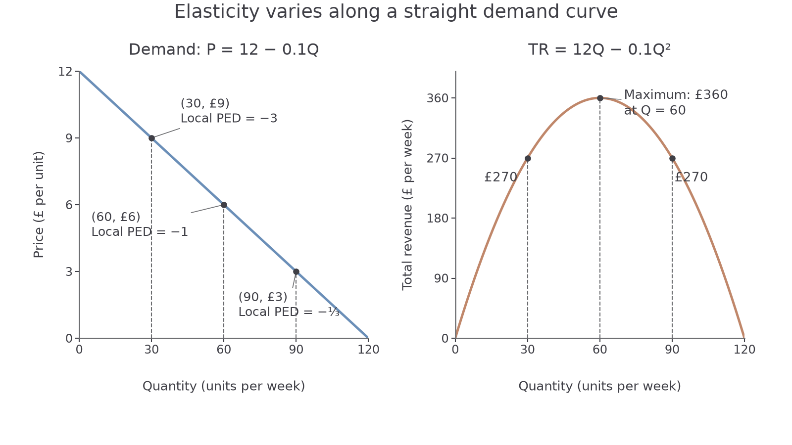
The demand schedule is illustrative: . Weekly TR is . At 60 units and £6, revenue reaches £360.
At 30 units and £9, a small price cut adds sales in the elastic region and increases revenue. At 90 units and £3, demand is inelastic: a small price cut loses more per existing sale than it gains from additional sales. The same straight line therefore changes elasticity as we move along it. Its constant slope does not imply constant PED.
Check an actual price change
For a finite change, calculate both revenues rather than treating the small-change relationship as an exact arithmetic rule. An illustrative seller changes price from £2 to £2.20 and quantity falls from 1,000 to 900. Using initial-value percentages gives PED . But TR changes from £2,000 to £1,980. The 10% price gain applies to only 900 remaining sales, so these finite changes do not exactly cancel.
If price changes by proportion and quantity by proportion , the exact revenue ratio is . Equal and opposite finite percentage changes leave a small product effect. A demand curve with constant unit elasticity has constant TR along it, but that claim is different from rounding one finite initial-value calculation to −1. Use the calculation convention and actual figures supplied by the task.
Notebook practice (ungraded): reproduce the two panels using the stated equations and the points (30, £9), (60, £6) and (90, £3). Label both axes, distinguish demand from revenue, and mark the revenue maximum. A typed explanation can show that you understand these relationships; it does not demonstrate that you drew the diagram.
Using an elasticity estimate
A useful pricing judgement links an elasticity estimate to the firm's objective and tests the conditions behind the estimate.
Suppose an illustrative cinema expects PED of −1.6 for weekday admissions. A modest price cut may raise TR because the predicted proportionate growth in tickets exceeds the proportionate fall in price. However, that does not establish higher profit: extra customers may require staffing, cleaning or another screening. A revenue-maximising choice can differ from a profit-maximising one.
The estimate may also come from an unsuitable comparison. Ticket sales might rise during a promotion because a popular film opens, not only because prices fall. An observed price–quantity pair then mixes an own-price response with a demand shift. The firm needs evidence that controls for relevant changes, or should treat the coefficient as uncertain.
Time, customer groups and capacity further affect the decision. A school-holiday estimate may not describe weekday adults. An average across buyers can conceal a highly elastic group and a less responsive group. If the cinema is already full, predicted extra demand cannot all become additional sales at that screening. A large price change may also enter a region with different elasticity, making a local estimate unreliable.
Consider the decision in a chain: the estimate predicts a response; that response affects sales and revenue; costs, capacity and the firm's objective determine whether the response is desirable. Then judge the evidence that supports the links. This is more informative than adding a list of unrelated “it depends” statements.
For example, a price cut is more convincing when spare seats are available, the estimate refers to similar weekday customers, rivals are unlikely to match it, and extra costs per admission are small. A cautious trial can reveal the response before a permanent change. A reasonable judgement can favour either a cut or keeping the price when the conditions support it; the numerical PED alone cannot settle every business decision.
Quick recap
PED compares percentage changes, with a negative sign for ordinary demand and an absolute value for responsiveness. Its determinants work through buyers' alternatives and adjustment opportunities. Link PED to revenue carefully, calculate finite changes directly, and check costs and evidence before using an estimate to choose a price.