4.1 - Perfect competition in the short and long run

Competition and price-taking

A perfectly competitive firm accepts the market price because customers can buy an identical product from many other suppliers.

Perfect competition assumes many buyers and sellers, a homogeneous product with no relevant differences between suppliers, good information about prices and products, and freedom of entry and exit in the long run. Each firm is too small to affect the industry price through its own output. Buyers can switch supplier without a meaningful obstacle. These assumptions explain behaviour; simply counting many firms is insufficient if each sells a distinctive product or customers cannot compare prices.

Industry demand and supply determine the market price. The individual firm faces perfectly elastic demand at that price: raising its own price loses its customers to identical substitutes. Charging less is unnecessary when it can sell its feasible output at the prevailing price. This horizontal firm demand is its average revenue (AR), and each extra unit earns the same price, so marginal revenue (MR) also equals price.

[DIAGRAM: asset_slug: h460-pc-price-taking; caption: Industry equilibrium determines the horizontal AR and MR faced by one small firm; description: Two illustrative panels with industry demand and supply crossing at price 6 and quantity 60, and firm AR equals MR equals price 6.]

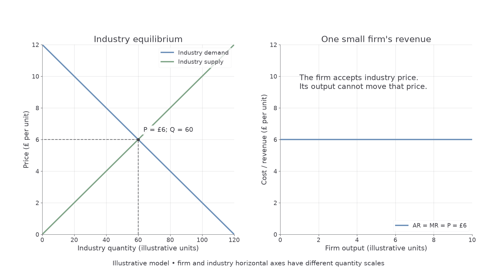
The left panel measures total industry quantity; the right measures one firm's quantity. The curves need not have comparable horizontal scales. A rise in industry demand can raise the price accepted by every firm, shifting each firm's horizontal AR and MR upwards. One firm's attempt to raise its price does not shift industry demand.

For a notebook diagram, put price or cost and revenue per unit on the vertical axis, quantity on the horizontal axis, and use separate industry and firm panels. Transfer the industry's equilibrium price across to the firm's horizontal AR=MR line. The firm is a price-taker, not a firm with no decisions: it still selects output and can change its costs.

Choosing profit-maximising output

A firm increases profit by adding a unit when its marginal revenue exceeds its marginal cost.

Marginal cost (MC) is the addition to total cost from another unit. When MR>MC, selling that unit adds more revenue than cost, so profit rises. When MC>MR, another unit lowers profit. The usual profit-maximising output therefore occurs where MC=MR on the rising section of MC, with MC moving from below MR to above it. A crossing on a falling MC section need not maximise profit. Discrete data may identify the last unit for which additional revenue covers additional cost rather than an exact equality.

In perfect competition MR=P, so the operating firm's output satisfies P=MC. Do not select output where AR meets average cost or where MC meets AC: those intersections answer different questions. Average cost (AC) includes all economic costs per unit, including the opportunity cost of the owner's resources. The firm earns normal profit when revenue covers these costs; normal profit is part of economic cost, not an extra surplus added afterwards.

An illustrative price-taking firm receives £9 per unit. Adding units with marginal costs £6 and £8 improves profit; an extra unit costing £11 reduces it. Its decision concerns the next unit, even if its average cost is £7. Total profit then requires total revenue and total cost, not MR minus MC alone.

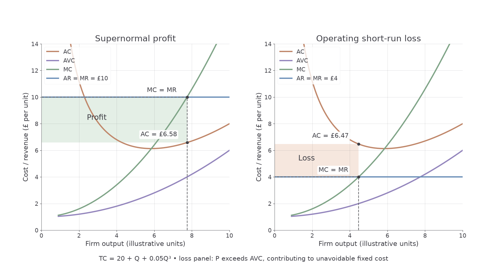
Once output is found, read price from the horizontal AR line and AC at that same output. Calculate $TR=P\times Q$, $TC=AC\times Q$, and economic profit $=(P-AC)Q$. If Q is measured in thousands, the resulting pound amounts are thousands of pounds. The method applies to both a positive profit and a loss.

Short-run profit and loss

In the short run, fixed factors and limited entry allow a price-taking firm to earn supernormal profit or make a loss.

Supernormal profit is revenue above all economic costs, including normal profit. If price exceeds AC at the MC=MR output, the profit rectangle has height P−AC and width Q. A firm can also face P<AC at its best output: choosing the smallest possible loss does not guarantee a positive profit.

[DIAGRAM: asset_slug: h460-pc-short-run; caption: At MC equals MR, price above AC gives profit and price below AC gives a loss; description: Cost-consistent short-run panels show a profit at price 10 and an operating loss at price 4, with the latter price above AVC.]