1.5 - Output gaps and economic fluctuations

Actual and potential output

An output gap is the difference between actual real output and the economy's potential output, the level sustainable without mounting inflationary pressure.

A negative output gap means actual output is below potential: usable labour and capital are underemployed. A positive output gap means actual output is temporarily above sustainable potential, often through exceptional hours and unusually intensive capacity use. Potential is an estimate of sustainable production, not necessarily the physical maximum that can be reached briefly. Normal frictional/structural unemployment can exist at potential, so potential does not mean literally every person working.

For illustrative potential output of £500 billion and actual output £480 billion, the gap is $(480-500)/500\times100=-4\%$. Actual output of £510 billion instead gives +2%. A gap changing from −4% to −2% narrows by 2 percentage points; the economy still has a negative gap. It has not moved into a positive gap merely because actual GDP grew. Potential can grow too, changing the denominator and the gap.

Potential cannot be observed directly as a single actual transaction. Estimates use trends, resource availability and productivity, and can be revised after a shock. If actual GDP falls 4% while sustainable capacity falls 5%, the gap may become more positive rather than more negative. Always compare actual with potential, instead of inferring the gap from the GDP growth rate alone.

Output gaps on AD–AS

An AD–AS diagram shows an output gap by comparing the current equilibrium's real output with the economy's potential output.

Put price level on the vertical axis and real output on the horizontal axis. Draw vertical LRAS at potential output Yp and an upward-sloping SRAS. A low AD curve can intersect SRAS to the left of LRAS at Y0; the horizontal distance Yp − Y0 is a negative gap. A sufficiently high AD curve can intersect SRAS to its right at Y2, a positive gap in the short run. Mark actual equilibrium points and their output projections; LRAS itself is not an additional equilibrium unless AD and SRAS intersect it.

[DIAGRAM: asset_slug: ocr_h460_output_gaps_adas; caption: Short-run equilibria below and above sustainable potential show negative and positive output gaps; description: AD–SRAS graph with potential 100, actual equilibria85,100,115 and labelled gaps on the real-output axis.]

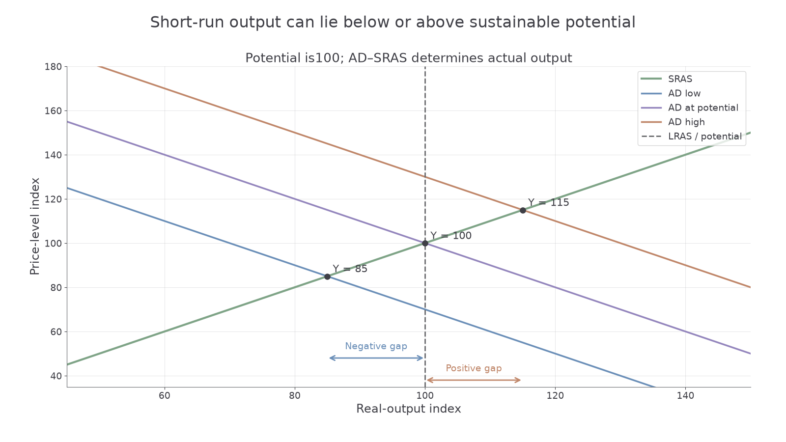
The graph does not depict a permanently feasible position beyond an unchanged long-run capacity. Above potential, longer hours and resource competition create wage and cost pressure. In the neo-classical adjustment model, rising costs shift SRAS left/up until output returns to potential at a higher price level. With deficient demand below potential, sticky wages and prices can slow recovery; low investment and prolonged unemployment may themselves damage future potential.

A supply shock can shift SRAS and LRAS. If energy availability permanently worsens, sustainable potential can fall as well as actual output. The left/right distance must then be measured from the new potential, rather than assuming every output reduction enlarges spare capacity.

Capacity on a PPC

A production possibility curve shows feasible combinations of two categories of real output using specified resources and technology.

Label the horizontal and vertical axes as quantities of two outputs, such as consumer goods and capital goods per year. A point inside the frontier can illustrate unemployment or inefficient use of existing resources. Moving towards a feasible point on the same frontier represents greater utilisation: actual output grows without an expansion of the underlying resource set. Moving along the frontier instead changes the mix, with opportunity cost; it does not by itself prove an output gap is closed.

[DIAGRAM: asset_slug: ocr_h460_gap_ppc; caption: Underused resources lie inside a PPC; points beyond a fixed feasible frontier require changed assumptions; description: Concave exact illustrative PPC, underutilised A, frontier B and infeasible C, axes consumer and capital goods per year, with no claim that a positive gap is permanently outside feasible capacity.]

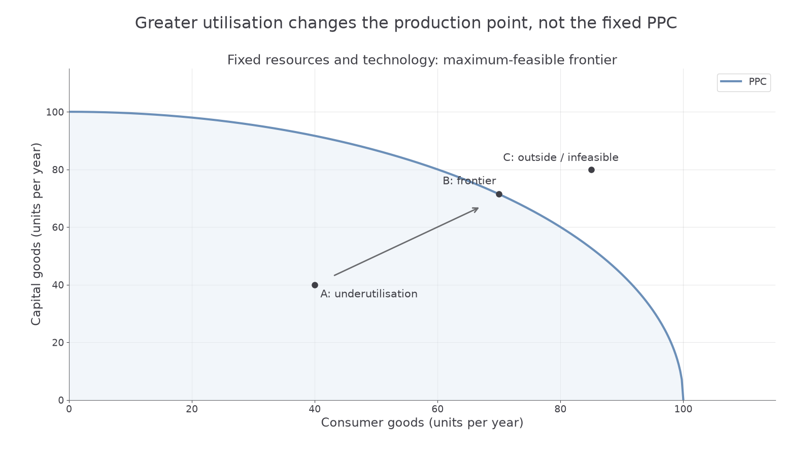
To construct the picture, draw a downward-sloping frontier bowed away from the origin to represent increasing opportunity cost, then mark A strictly inside and B on it. C outside is infeasible under the stated fixed resources and technology. It must not be labelled as an ordinary permanently attainable positive output gap. A sustainable-capacity benchmark may be drawn inside an exceptional short-run physical limit: temporary overtime could push production above that benchmark while remaining physically possible. If the PPC is defined as the maximum feasible output, a move outside requires a changed resource/technology assumption, rather than merely extra demand. This distinction reconciles PPC feasibility with the AD–AS concept of output temporarily above sustainable potential.