2.6 - Price elasticity of supply

Calculating PES

Price elasticity of supply measures the proportional response of quantity supplied to a change in a good's own price, other supply influences held constant.

In an illustrative bakery, price rises from £2 to £2.20 per loaf and planned weekly supply rises from 1,000 to 1,150 loaves. Price rises 10%; quantity supplied rises 15%; PES is $15/10=1.5$. This is elastic supply: quantity responds more than proportionately. For $0<\mathrm{PES}<1$, supply is inelastic; at 1 it is unit elastic. PES is a ratio without units, not the number of extra loaves per pound.

PES is normally non-negative because a higher price increases the profitability of additional production. A fall in price and a fall in quantity give two negative changes whose ratio is positive. If observed price and quantity move oppositely because a harvest fails, that is likely a supply shift, not evidence of negative elasticity along an unchanged supply curve. In calculations, distinguish quantity supplied from quantity demanded and from an output change caused by new technology.

Supply diagrams and values

Supply diagrams place the product's price vertically and quantity supplied horizontally, so their slope is not itself elasticity.

To construct a model, label price per unit and quantity per stated period, plot price–quantity combinations and draw the supply curve through them. A perfectly inelastic supply curve is vertical: available quantity is fixed when price changes, so PES is 0. A perfectly elastic curve is horizontal: the model makes any amount available at one price; an arbitrarily small price increase induces a very large quantity response. Infinite elasticity is a limiting model, not a ratio calculated from two identical prices.

[DIAGRAM: asset_slug: pes-values; caption: Inelastic, unit-elastic and elastic supply compared with perfect limiting cases; description: Exact power-function supply curves through a common price–quantity point, with local PES 0.5,1,2 and vertical/horizontal limiting cases.]

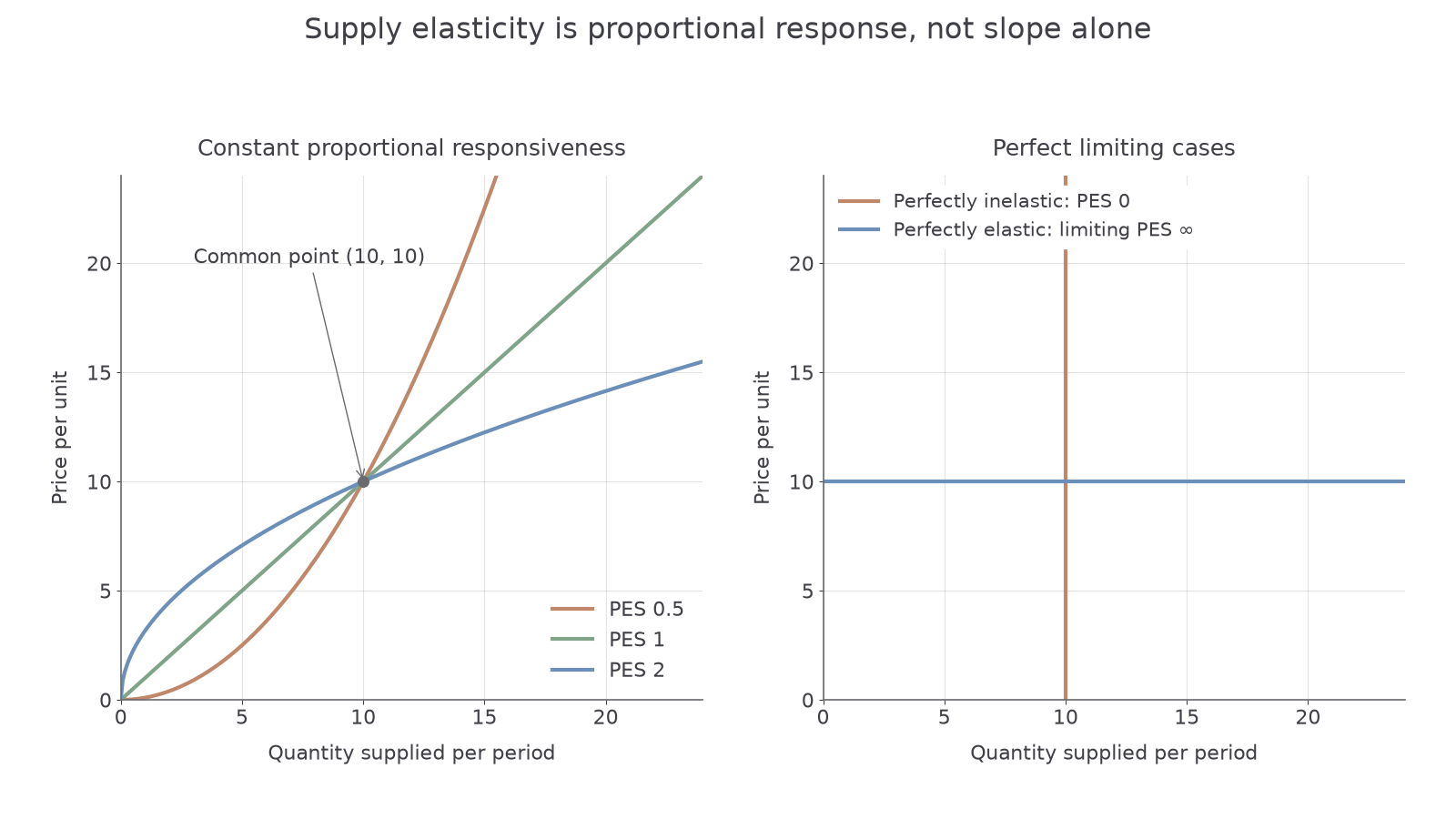
The first panel compares supply functions through quantity 10, price 10. $Q=10(P/10)^{0.5}$ has PES 0.5, $Q=P$ has PES 1, and $Q=10(P/10)^2$ has PES 2 at positive prices. In this comparison the elastic curve is flatter near the common point. Without shared axes, units and a comparable point, calling one curve flatter is insufficient: elasticity is proportional responsiveness, whereas slope changes if pounds become pence.

For a straight upward supply curve, local PES is $(dQ/dP)(P/Q)$. A straight ray from the origin has PES 1 all along it, whatever its positive slope. A straight curve crossing the price axis above the origin has PES greater than 1 at positive quantities; one crossing the quantity axis to the right of the origin has PES less than 1. These statements assume the normal upward linear segment and positive price and quantity. A large finite initial-base calculation can differ from the local value on a curved supply function.

Why supply responsiveness varies

Supply is more responsive when producers can add saleable output quickly without sharply increasing the cost of each extra unit.

Spare capacity allows an existing factory to add shifts or use idle machines. If every machine is already fully used, expansion may need a new building and supply responds little immediately. Stocks of finished goods can be released quickly after a price rise, making market supply more elastic than current production; fresh fruit cannot be stored as long as canned food. Factor mobility matters: firms expand more easily when suitable workers, equipment and materials can move into the activity. Training requirements, specialist machinery and scarce land slow the response.

The time period changes these constraints. In the very short run a completed crop is largely fixed. Over the next season farmers can change planting; over several years they may acquire land or irrigation. Supply therefore often becomes more elastic over time, but it need not: environmental limits or a fixed site can remain binding. A highly perishable product with limited storage may have inelastic supply even when producers want to expand. Assess the actual bottleneck rather than treating time as an automatic guarantee.

In an illustrative clothing firm, an unexpected price rise can be met by drawing down stocks today. A sustained rise can justify hiring and expanding machinery later. If fabric imports are disrupted, both responses can be weaker than an old PES estimate suggests because the supply curve itself also shifts. PES asks about a price-induced movement along a curve under specified conditions.

Using PES in decisions

PES helps predict whether a change in demand will mainly change a market's price or its quantity, and whether a production policy can expand output.

Consider a rightward demand shift with no supply shift. If supply is very inelastic, firms add little output; competition for the limited quantity mainly raises price. More elastic supply allows a larger output increase and limits the price rise. This helps explain why housing demand can initially raise prices strongly where building is slow, while easily manufactured goods may expand more rapidly. It does not prove any particular price change without demand and supply data.

A per-unit subsidy lowers producers' marginal cost and shifts supply down. With demand held fixed, the output and buyer-price effects depend on both elasticities. In the usual competitive model, relatively inelastic supply gives producers a larger share of a subsidy and leaves output relatively unresponsive; elastic supply transmits more towards lower buyer prices and expansion. Similarly, a relatively inelastic side of a market bears more of a specific tax. These are comparisons of relative demand and supply responsiveness, not rules that PES alone determines every burden.

An estimate can help a government judge whether a subsidy for an essential product is likely to increase availability or mainly raise producer receipts. Yet a value estimated before a capacity limit, input disruption or regulatory change may not apply. A short-run estimate is unsuitable for a ten-year infrastructure decision. Combine recent evidence with the relevant time horizon and bottleneck; changing capacity may be more useful than paying for extra production the firm cannot deliver. A higher elastic response also says nothing by itself about external costs or whether the resulting quantity is socially efficient.

Quick recap

PES measures percentage quantity response to percentage own-price change. Capacity, storage, mobility and time shape that response. Interpret diagrams in consistent units and use estimates with the relevant demand conditions and time horizon.