2.6 - Income and cross elasticity of demand

Measuring income elasticity

Income elasticity measures the responsiveness of quantity demanded to a change in consumers' income, holding the good's price and other demand influences constant.

Income elasticity of demand (YED) is a ratio of two percentage changes. It has no units: dividing percentage by percentage removes the scale. The sign conveys the direction of the response, while the magnitude conveys its relative size.

In an illustrative survey, monthly income rises from £2,000 to £2,200 and demand for restaurant meals rises from 10 to 12 per month. Income rises by $200/2000\times100=10\%$; quantity rises by $2/10\times100=20\%$. YED is $20/10=+2$. Over this change, a 1% income rise is associated with a 2% quantity rise. It does not mean two extra meals for every extra pound. If income had fallen, use its negative percentage change consistently; do not remove signs before dividing.

An estimate from sales and income moving together is not automatically a causal estimate: a restaurant price cut, population growth or changing tastes could also raise sales. An experiment or statistical estimate must separate these influences before the YED can support a reliable forecast.

Normal and inferior goods

The sign of YED distinguishes goods whose demand rises with income from goods whose demand falls with income.

A normal good has positive YED: higher income raises quantity demanded, other things equal. For $0<\mathrm{YED}<1$, demand is income inelastic; spending may rise but quantity rises less proportionately than income. Such goods are often called necessities. For $\mathrm{YED}>1$, demand is income elastic, often described as a luxury. At +1, quantity and income change in the same proportion. YED of zero means no quantity response to the income change in that range.

An inferior good has negative YED. When income rises, some buyers switch away from it towards preferred alternatives. This is about observed choices, not product quality or whether a good is harmful. A cheap bus journey might be inferior for commuters who buy a car after an income rise, yet normal for other households. Classification can change across income ranges, places and time.

An Engel curve plots quantity demanded against income while other influences are fixed. To construct the following model, put monthly income on the horizontal axis, quantity per month on the vertical axis, plot pairs and join them smoothly. An upward relationship represents a normal good and a downward one an inferior good. With these axis choices, proportional responsiveness is slope multiplied by income/quantity; a steep curve alone does not identify YED. The plotted functions show constant YED values over positive incomes, making the comparison precise.

[DIAGRAM: asset_slug: yed-engel; caption: Engel curves for income-inelastic normal, income-elastic normal and inferior goods; description: Three exact quantity-income functions with constant YED +0.5, +2 and −0.5, at positive incomes.]

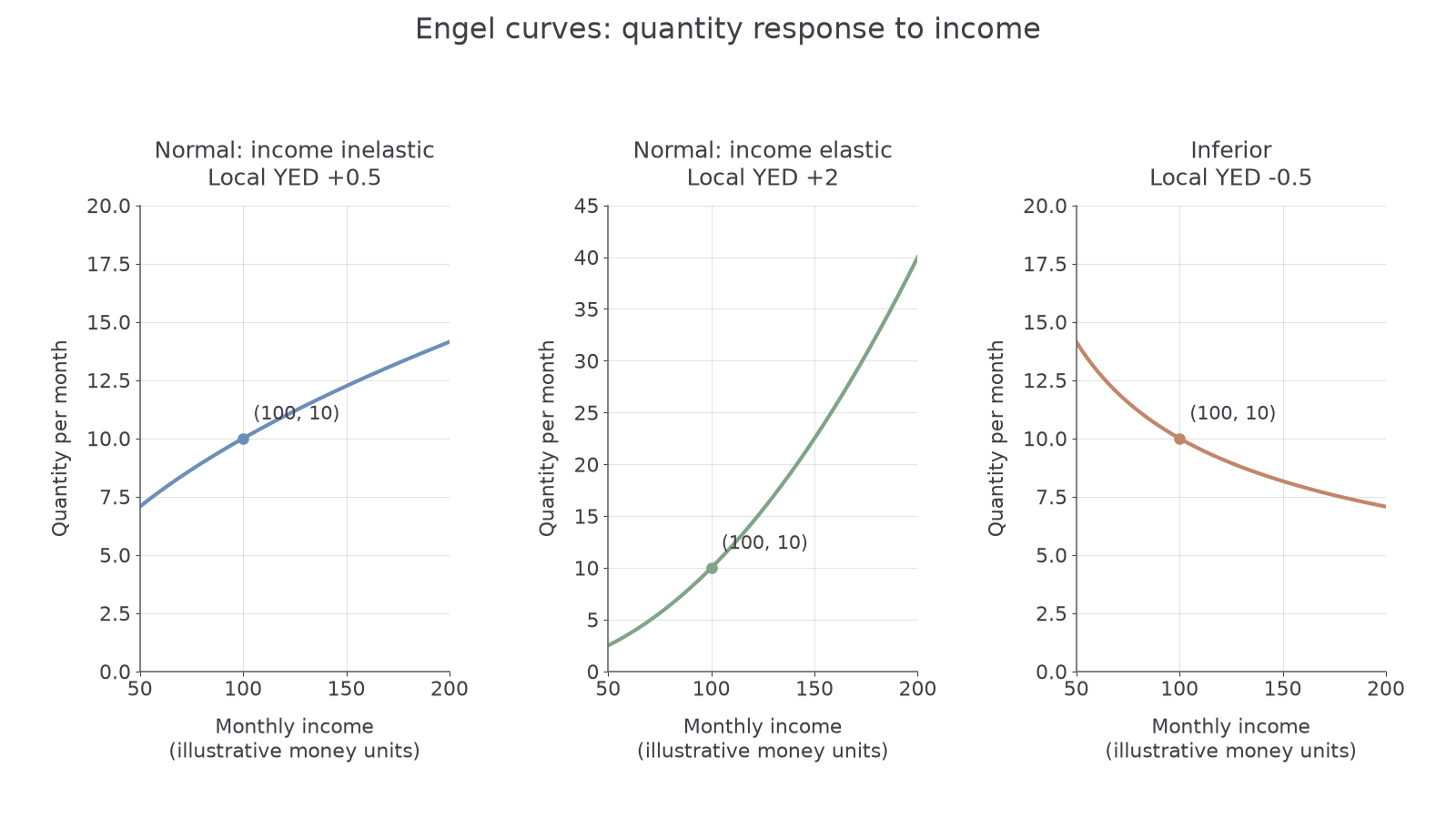
For example, from income 100 to 121, quantity on the YED +0.5 curve rises from 10 to 11. The finite initial-base estimate is $10\%/21\%\approx0.48$, close to, but not exactly, its point elasticity +0.5. The graph's labels describe local proportional responsiveness. Larger finite changes can give a different initial-base estimate; never assume a curve's visual slope is its elasticity.

Measuring cross elasticity

Cross elasticity measures how demand for one good responds to a change in the price of another good.

Keep the goods in the right places: the numerator concerns quantity of A and the denominator price of B. Hold A's own price, incomes and other demand influences constant. In an illustrative case, the price of coach journeys rises from £20 to £22 and demand for rail journeys rises from 500 to 540. The changes are +10% and +8%, so rail demand's XED with respect to coach prices is $+8/+10=+0.8$.

Substitutes have positive XED: when B becomes dearer, customers switch towards A. Complements have negative XED: when B becomes dearer, demand for B falls and demand for goods used with it also falls. If game consoles rise in price by 10% and game demand falls by 6%, games' XED with respect to console prices is −0.6. Unrelated goods have XED near zero. A zero estimate can also conceal offsetting influences or weak data, so it is evidence about a measured response rather than proof of no possible connection.

Greater absolute XED indicates a stronger proportional response over the relevant range. It need not exceed 1 to indicate substitution or complementarity. XED of A with respect to B need not equal XED of B with respect to A: spending shares, alternatives and consumer groups differ.

Showing related-market responses

A related-price graph shows quantity of A against the price of B, rather than the own-price demand curve for A.

Construct the response graph with price of B on the horizontal axis and quantity of A on the vertical axis, keeping A's own price fixed. The substitute curve slopes up, the complement curve slopes down, and an unrelated response is horizontal. The following curves have constant local XED +1, −1 and 0. Their shapes describe this axis choice; a complement response is not an own-price demand curve simply because both slope down.

[DIAGRAM: asset_slug: xed-responses; caption: Cross-price responses for substitutes, complements and unrelated goods; description: Quantity of A against price of B, with constant local XED +1, −1 and 0.]

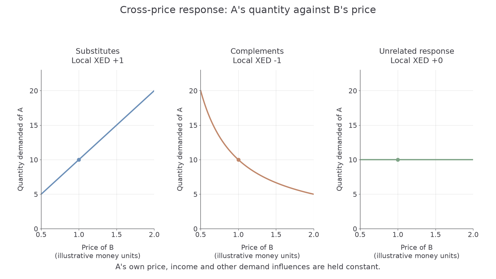
On a conventional market diagram for A, put A's own price vertically and quantity of A horizontally. A rise in the price of substitute B shifts A's demand curve right at every own price; supply is unchanged and the new equilibrium normally has higher price and quantity. A rise in the price of complement B shifts A's demand left, normally lowering both. It is a shift of demand for A, not a movement along that curve. The resulting equilibrium quantity response also depends on A's supply elasticity: XED measures the demand response with A's own price held fixed, whereas market sales incorporate the subsequent price adjustment.

For a numerical illustration, at A's fixed price £5 a rise in B's price changes desired purchases from 100 to 120. Mark the two quantities on separate demand curves at £5. Do not label 120 as the final traded quantity unless the supply conditions actually keep A's price at £5.

Using elasticity estimates

Elasticity estimates help a firm forecast demand, but their usefulness depends on the consumers, range and conditions from which they were estimated.

YED depends on the role a good plays in a household budget and on income. Basic food may respond little once nutritional needs are met, while expensive holidays can be postponed. A good can become less income elastic as households become richer and approach a desired level of consumption. XED depends on the closeness and availability of substitutes or complements: two frequent routes between the same cities may be close substitutes, while routes at different times may serve different buyers. Adjustment time matters because customers need time to find alternatives or replace durable goods. Brand attachment and switching costs can weaken a substitute response.

Suppose an illustrative holiday firm's YED estimate is +1.8 and household income is forecast to rise 3%. A first forecast is quantity growth $1.8\times3\%=5.4\%$. Capacity and staffing can be planned around that possibility. Conversely a recession can reduce income-elastic demand sharply; necessity sellers may face a smaller fall. With XED +0.6, a rival's forecast 10% price cut implies about 6% lower demand for the firm at its unchanged own price. That could inform promotion or product differentiation. A complement producer may coordinate bundles or anticipate a partner's price change.

The forecast is conditional, not a promise. An old estimate may cover a different income range or market; a recession can change confidence as well as income. Simultaneous own-price changes and supply constraints mean the estimated demand shift is not identical to actual sales. A firm should use recent evidence, test several forecasts and compare forecast errors before committing to expensive capacity. A close substitute's positive XED is useful competitive evidence, but on its own does not prove a legal market boundary or how every consumer will react.

Quick recap

YED compares quantity with income; XED compares quantity of one good with another good's price. Keep the signs, percentage bases and fixed conditions clear. Diagrams and forecasts are useful only when their variables and assumptions match the decision.