1.5 - The multiplier and accelerator

Average and marginal propensities

A propensity is a ratio describing how income is used; an average ratio uses total levels, whereas a marginal ratio uses changes.

For a household, define Yd as disposable income, C as consumption and S as saving. If all disposable income is consumed or saved, $Y_d=C+S$. Then APC, the average propensity to consume, is $C/Y_d$, and APS is $S/Y_d$. They sum to one under this definition. A household with annual disposable income £30,000, consumption £24,000 and saving £6,000 has APC = 0.80 and APS = 0.20. These are 80% and 20% shares, not percentage changes in consumption.

The MPC is $\Delta C/\Delta Y_d$, and the MPS is $\Delta S/\Delta Y_d$. If disposable income rises by £2,000, consumption rises by £1,500 and saving rises by £500, MPC = 0.75 and MPS = 0.25. Marginal ratios need not equal average ratios. When comparing observations, take the change in each variable first and use the same time period and income definition. A fall in both income and consumption can also give a positive MPC: two negative changes divide to a positive ratio.

For national-income models below, Y means income before the defined net-tax leakage. The average propensity to withdraw APW is $(S+T+M)/Y$, while the marginal propensity to withdraw MPW is $\Delta(S+T+M)/\Delta Y$. Saving, taxes and imports must be defined consistently so they do not overlap. At annual national income £500 million, S = £40 million, T = £100 million and M = £60 million give APW = 200/500 = 0.40. If an extra £100 million of income generates extra S = £10 million, T = £20 million and M = £15 million, MPW = 45/100 = 0.45. The average withdrawal share and marginal withdrawal share therefore differ. The remaining marginal fraction 0.55 supports induced expenditure on domestic output in this simplified model. A household MPC out of disposable income is not automatically that domestic-spending fraction: taxation and imports must also be allowed for.

Successive spending rounds

The national income multiplier is the ratio of the total change in national income to the initial autonomous spending change that caused it.

Autonomous spending is spending not induced by the current income change. Suppose an extra £10 million of government purchases pays domestic producers, with spare resources and stable prices. Those receipts become wages and profits; recipients spend part of their extra income on domestic output, generating income for others. If the induced domestic-spending fraction is 0.60, the initial £10 million is followed by £6 million, £3.6 million, £2.16 million and successively smaller rounds. Each round is another producer's income; the total includes the original £10 million. It is not a claim that each pound physically passes round the economy exactly five times.

Leakages stop each round being as large as the last. The series is $10+10(0.60)+10(0.60)^2+\cdots$, tending to £25 million. The eventual extra income is therefore 2.5 times the initial injection. The initial injection is not multiplied by 2.5 and then added again: that would double count it. A spending cut works in the reverse direction under the same assumptions, causing lower income and further spending reductions.

[DIAGRAM: asset_slug: ocr_h460_multiplier_rounds; caption: Successive domestic spending rounds shrink, while their cumulative income effect approaches £25 million; description: Exact plot of10(0.6)^n spending rounds and cumulative geometric-series income, with axes labelled round number and £million.]

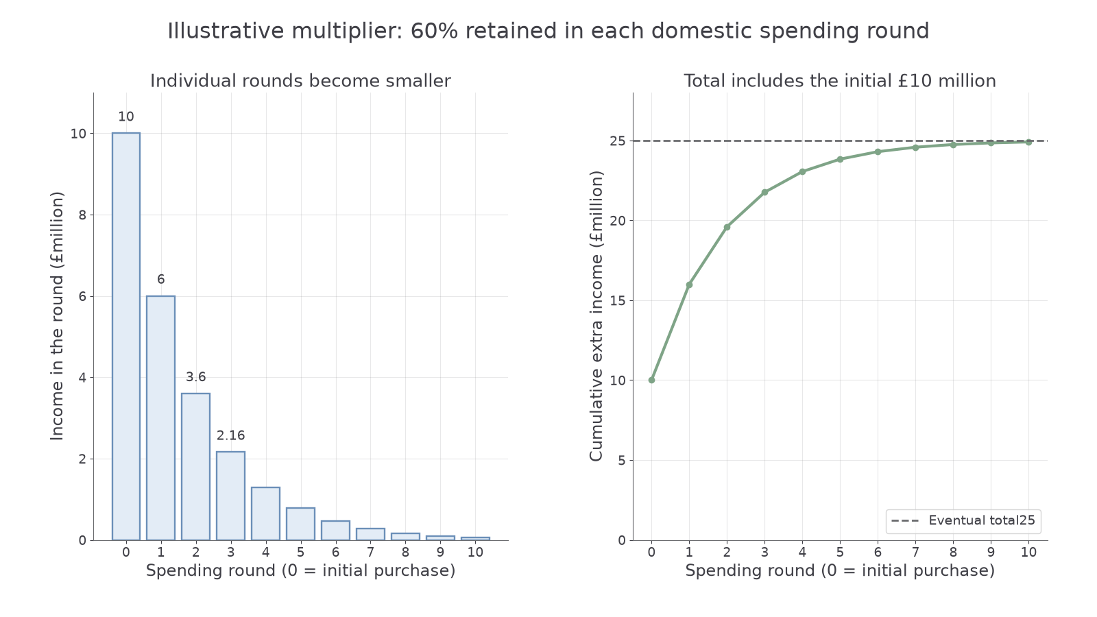
The horizontal axis counts spending rounds, not necessarily equal months. The vertical axes show amounts of income, not a growth rate. In a notebook, calculate each round by multiplying the previous one by the retained domestic-spending fraction, then plot the separate amounts and cumulative sums. Time lags mean a textbook eventual effect need not appear immediately in measured quarterly GDP.

Calculating the multiplier

The multiplier becomes smaller when more of each additional unit of income leaks from spending on domestic output.

With a constant MPW, fixed prices and sufficient spare capacity, the simplified open-economy multiplier is:

In a closed economy without government, income is either consumed or saved and there are no tax/import leakages. Only in that simpler case is $k=1/\mathrm{MPS}=1/(1-\mathrm{MPC})$, where MPC is out of that same income. If MPC = 0.80, MPS = 0.20 and k = 5. Applying 1/(1 − household MPC) to an open economy without accounting for taxes/imports can overstate the effect.

For an illustrative open economy, an income increase of £200 million produces extra saving £20 million, net taxes £40 million and imports £20 million. MPW = 80/200 = 0.40, so k = 2.5. An autonomous domestic investment increase of £12 million gives a modelled eventual income increase of £30 million. If MPW rises from 0.40 to 0.50, k falls to 2. Saving/tax/import responses can change as income changes; assuming a constant ratio is a modelling choice. A multiplier is a ratio, not a money amount.