2.3 - Supply and related production
Supply describes what producers are willing and able to offer for sale at different prices. Learn how incentives and production costs affect that relationship, how firms' supplies form market supply, and why producing one good can change the supply of another.
Price and quantity supplied
A supply curve shows quantities offered for sale at different own prices during a stated period, holding other relevant influences constant.
An ordinary upward-sloping supply curve reflects the incentive to expand output when a higher price makes additional production worthwhile. Expanding within existing facilities may require overtime or less suitable inputs, raising the cost of extra units. A higher price can cover those costs. The relationship is about willing and able supply: a firm cannot instantly offer unlimited output just because price rises.
In an illustrative weekly schedule, over the plotted range. At £2, quantity supplied is 6 units; at £4 it is 14; at £6 it is 22. Plot quantity horizontally and price vertically, label both units and the period, then join the points with S. Supply is a flow offered over time, not simply the stock stored in a warehouse.
A rise in own price from £2 to £4 causes an extension of supply from 6 to 14 along S. A price fall causes a contraction. These are changes in quantity supplied along the unchanged price–quantity relationship. They are not an increase or decrease in the whole supply curve.
[DIAGRAM: asset_slug: h460-foundations-supply-move; caption: A higher own price extends supply along S, while lower production costs shift S right; description: Two exact illustrative supply panels, original Q4P minus2, movement from P2 Q6 to P4 Q14, and shifted Q4P plus4 showing Q14 to20 at fixed P4.]
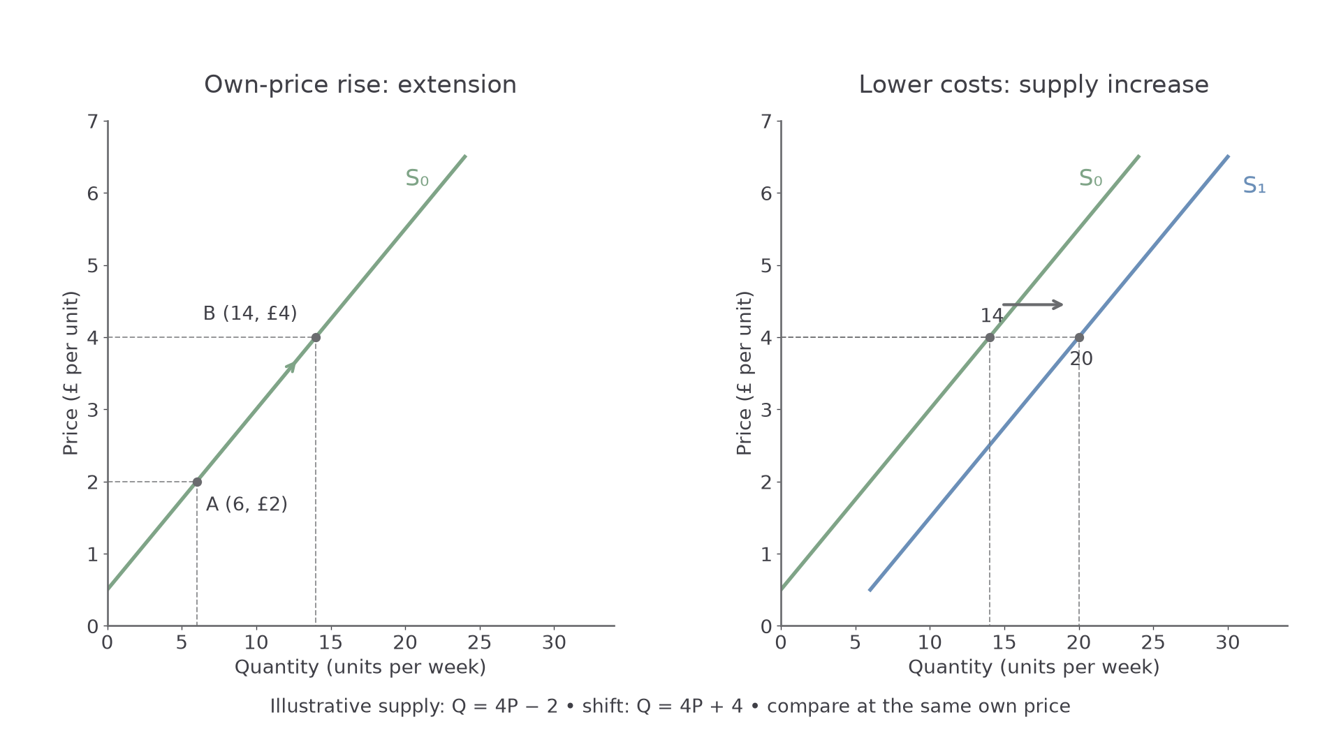
The left panel changes own price. The right panel changes a non-price influence, so firms offer more at each possible price.
Individual and market supply
Market supply adds the quantities supplied by all producers at each common price.
For two illustrative firms, A supplies 4 units and B supplies 2 at £2, giving market supply of 6. At £4 their supplies are 8 and 6, giving 14. At £6 they are 12 and 10, giving 22. This is horizontal summation: add quantities at the same price, for the same good and period. Do not add different firms' selling prices.
[DIAGRAM: asset_slug: h460-foundations-market-supply; caption: Horizontal summation combines quantities supplied by A and B at a common price; description: Three exact illustrative curves A Q2P, B Q2P minus2 and market Q4P minus2 for price1to6, highlighting at P4 quantities8 plus6 equals14.]
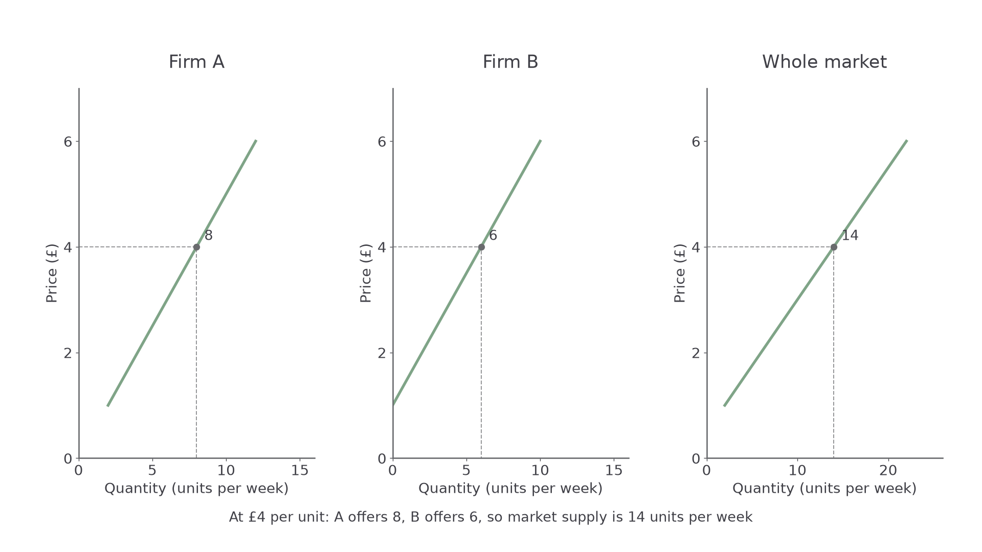
At £4, A offers 8 and B offers 6 units per week, so the whole two-firm market offers 14.
To construct the market curve, build a price table, add each row's individual quantities and plot the total. If a firm supplies nothing below its relevant threshold, use zero rather than extending a mathematical line into negative output. Entry of additional producers can shift market supply right even if every existing firm's curve is unchanged. A firm closing can reduce market supply.
The horizontal sum is an accounting relationship at each price. It does not imply producers have identical costs, capacities or technologies. Nor does it determine the actual price; that requires demand as well as supply.
Shifts of supply
A non-price influence shifts supply when it changes the quantity firms offer at each possible own price.
An increase in supply shifts S right; a decrease shifts it left. Lower input costs can make additional production profitable at a given selling price. Higher wages or energy prices, with other conditions unchanged, can reduce supply. An improvement in technology that reduces the resources needed per unit can increase supply; whether a particular new technology lowers cost requires evidence rather than its label alone.
Taxes on production or sales can raise the relevant private cost and shift supply left or up; a per-unit subsidy can reduce it and shift supply right or down. The details of tax and subsidy diagrams are taught in 2.11. Weather and natural conditions can affect agricultural yields. Entry, exit and available capacity can change market supply. Expectations may cause producers with storable goods to withhold current output in anticipation of a higher future price, though this is not possible for every service.
In the right panel, illustrative supply changes from to . At £4, supply rises from 14 to 20. This fixed-price comparison identifies the shift; it does not claim actual equilibrium price remains £4.
Suppose an illustrative bakery's flour price rises while bread's selling price initially stays the same. Higher costs reduce the bread output worth offering at that price: bread supply shifts left. If bread's own price later rises as the market adjusts, that causes a movement along the new supply curve. Cost and own-price effects must not be confused.
Joint and competitive supply
Supply relationships connect goods through the production process or through competing uses of the same resources.
Joint supply occurs when producing one good also produces another, such as beef and hides used for leather. If higher beef demand makes cattle production expand, more hides can become available, shifting hide supply right at each hide price. The relationship depends on the technology and how usable the by-product is. The quantity of hides is tied to cattle production, so its producer cannot always adjust it independently like an unrelated product.
Competitive supply occurs when goods compete for the same resources. An illustrative farmer can use a field for wheat or barley. If wheat becomes more profitable, land can switch from barley to wheat. Barley supply then shifts left at each barley price. This is distinct from competitive demand, where consumers switch between substitutes: here producers reallocate inputs between outputs.
[DIAGRAM: asset_slug: h460-foundations-related-supply; caption: Joint production can expand a by-product's supply, while competing production can reduce another good's supply; description: Exact illustrative hide-supply shift right after greater cattle production and barley-supply shift left after land switches towards wheat, holding the affected goods own prices at4.]
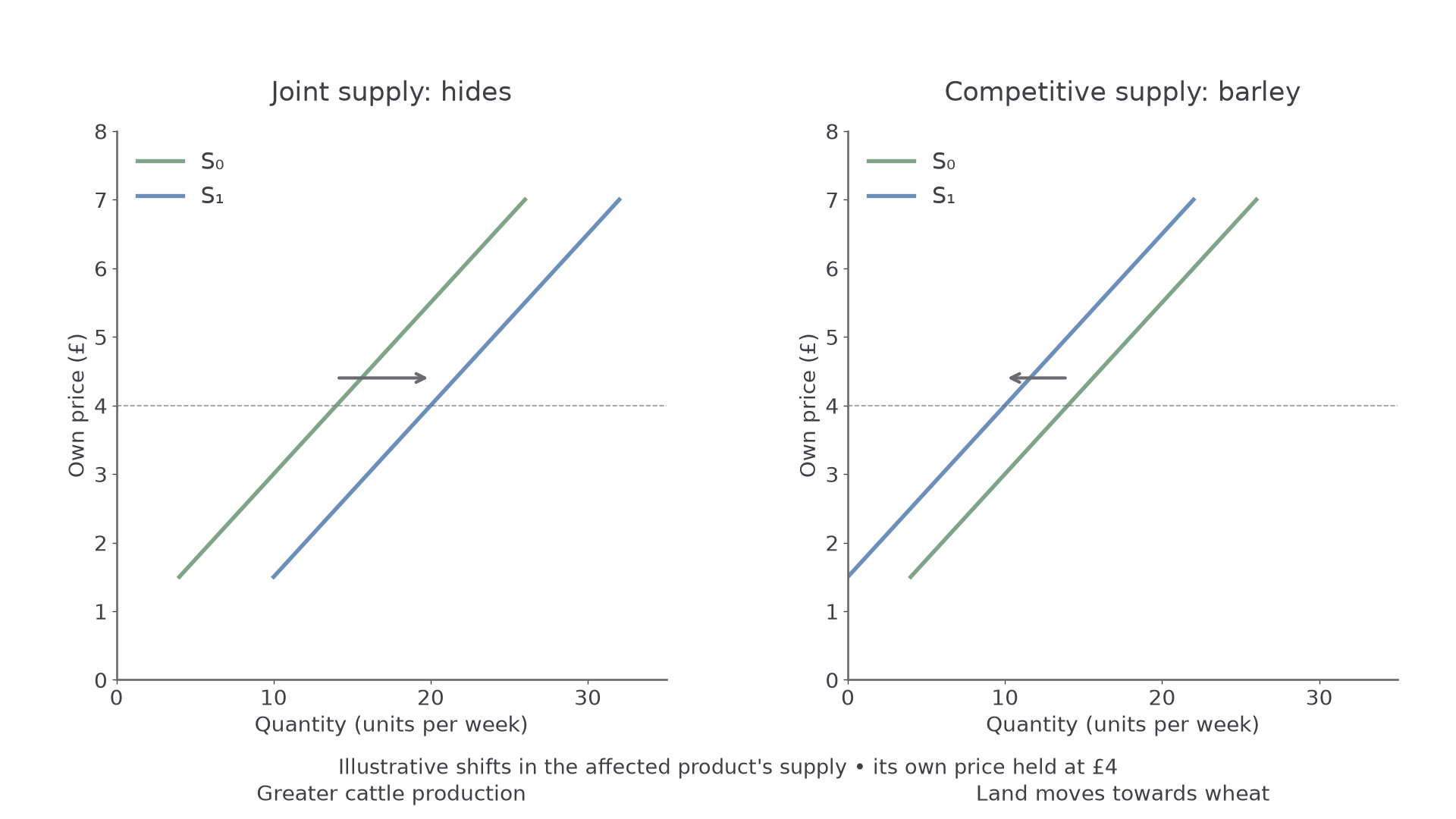
Each panel names the affected product. An incentive elsewhere in production changes the quantity offered at a common own price.
The strength and speed of these effects depend on resource mobility. Land may be unsuitable for the alternative crop, workers may need retraining and equipment may take time to replace. A wheat-price rise therefore need not immediately cut barley supply by a fixed amount. Similarly, more cattle only expands usable hide supply if collection and processing capacity can handle the extra output.
For a notebook diagram, label the affected good on both axes, draw S0 and S1 and show quantities at the same own price. Put the cause in a caption rather than shifting a curve without naming the market. In a connected-market explanation, distinguish the first market's own-price movement from the second market's non-price supply shift.
Quick recap
Own-price changes move quantity supplied along S; non-price cost or production changes shift it. Market supply adds firms' quantities at common prices. Joint products and competing resource uses explain how another market can change the affected good's supply.