3.2 - Short-run costs and diminishing returns
Producing more can reduce the cost per item at first, then make each extra item increasingly expensive. Learn to calculate total, average and marginal costs, and to explain their shapes using fixed factors and diminishing returns in the short run.
Fixed factors and cost categories
The short run is a period in which at least one factor of production is fixed. The long run is a period in which all factors can be varied. These are possibilities for adjustment, not fixed calendar lengths: fitting out a new factory can take much longer than expanding a small online service. A bakery with a fixed oven can add labour or ingredients in the short run, but cannot immediately double its oven capacity.
Total fixed cost (TFC) does not change with output within the relevant range. Rent on the existing premises is a typical example. Total variable cost (TVC) changes with output; flour and labour paid according to the production required can be examples. Classification depends on the actual contract and time period. A salaried worker's pay need not vary with today's output, while an overtime payment may do so. Fixed does not mean permanently unchangeable, and variable does not mean proportional to output.
Total cost
At zero output, variable cost is zero in the basic model, while fixed cost remains payable. If illustrative daily rent is £60 and producing four batches requires £80 of variable inputs, total cost is £140. If output doubles, rent can remain £60 but input costs need not merely double: congestion may make labour hours per batch rise. In the long run, a firm can alter or leave its premises; there is no fixed factor in that definition.
Average and marginal cost
An average cost divides a total cost by output. Marginal cost (MC) is the additional total cost of additional output. It answers a different question from average cost: “What does the next unit add?” rather than “What does each unit cost on average?”
For discrete output changes, . With fixed cost unchanged, . At zero output, average cost is undefined: division by zero is not a cost of zero.
This illustrative bakery table measures output in batches and money in pounds per day:
| Batches Q | TFC | TVC | TC | AFC per batch | AVC per batch | ATC per batch | MC of latest batch |
|---|---|---|---|---|---|---|---|
| 0 | 60 | 0 | 60 | — | — | — | — |
| 1 | 60 | 30 | 90 | 60 | 30 | 90 | 30 |
| 2 | 60 | 50 | 110 | 30 | 25 | 55 | 20 |
| 3 | 60 | 60 | 120 | 20 | 20 | 40 | 10 |
| 4 | 60 | 80 | 140 | 15 | 20 | 35 | 20 |
| 5 | 60 | 120 | 180 | 12 | 24 | 36 | 40 |
At Q = 4, ATC is £140/4 = £35 per batch, but MC is (£140 − £120)/(4 − 3) = £20. The fourth batch costs less than the previous average, so ATC falls from £40 to £35. The fifth batch costs £40, more than the previous average £35, so ATC rises to £36. Discrete tables do not require the measured MC number to equal the minimum measured ATC exactly; the exact crossing rule applies to smooth curves.
Average fixed cost keeps falling as fixed cost is spread over more output. This alone does not guarantee falling ATC: a sufficiently large rise in AVC can outweigh it. At Q = 5, fixed cost is one-third of total cost (£60/£180), and variable cost is two-thirds. TVC rises from £80 to £120, a increase, while output rises only 25%. Use the initial cost as the percentage base; £40 is an absolute increase, not 40%.
Diminishing marginal returns
The law of diminishing returns says that, as successive units of a variable factor are added to fixed factors, the extra output produced eventually falls, assuming unchanged technology and comparable input quality. This is diminishing marginal product, not necessarily falling total output. Marginal product is the extra output from an extra unit of the variable factor.
With a fixed kitchen, the first extra workers can specialise: one prepares dough while another operates the oven. Marginal product may initially rise. Eventually the oven and workspace become bottlenecks. Extra workers spend longer waiting, so each adds less output even though total output still rises. Only when marginal product becomes negative does adding workers reduce total output, for example through severe interference. The law concerns the eventual stage; it does not require an initial stage of increasing returns or negative marginal product within every practical range.
[DIAGRAM: asset_slug: diminishing-returns; caption: Total product and marginal product with a fixed factor; description: Illustrative total product increases while marginal product eventually falls; total product reaches its maximum where marginal product is zero.]
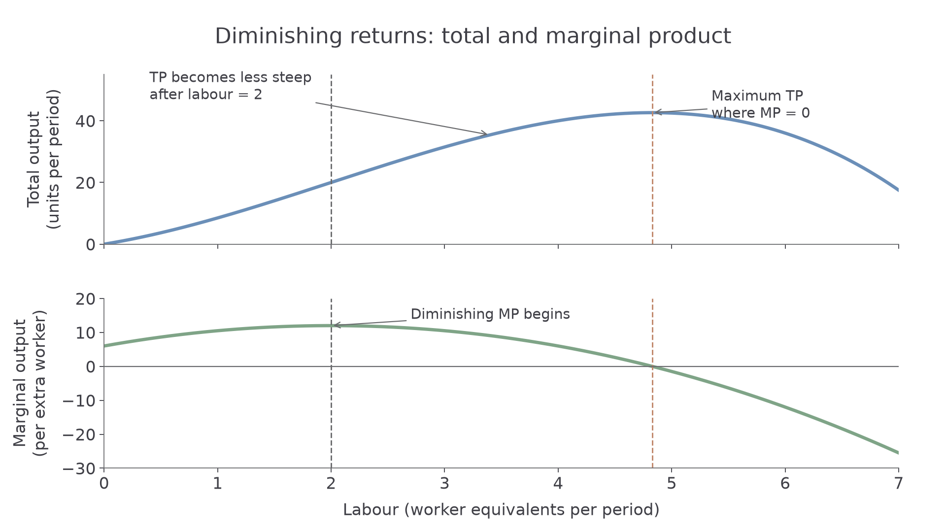
In the upper panel, labour per period is on the horizontal axis and total output per period on the vertical axis. The curve becomes steeper while marginal product rises, then becomes less steep as marginal product falls. The lower panel places labour against marginal output per extra unit of labour. Its peak marks the point after which diminishing marginal returns begin. Its zero corresponds to the maximum of total product. The plotted values are an illustrative smooth model, not estimates for an actual bakery.
Continue this lesson.
You’re previewing NovaLearn without an account. Create a free account to read the rest.
Create free account