Appendix 2 3, 4; 9GE0/04 - Physical fieldwork measurements and data quality

Observations, indicators and site records

Physical fieldwork measures indicators of processes, so an observed form and an inferred explanation must be distinguished.

A beach profile records shape at the survey time. It does not directly measure the annual sediment budget. A channel cross-section records width and depth at a place and time; it does not alone establish a river's annual flood regime. Select observations that relate to the enquiry, then identify the additional context or repeats needed for its intended timescale.

Locate sampling sites using a consistent map reference or coordinates and a stated coordinate system. A field sketch records significant features, relative positions and observation direction; a scale or dimensions should be included where relevant. An annotated photograph can retain evidence of vegetation, surface conditions or a structure. Label date, location, direction and scale, and distinguish what is visible from what you infer. Respect permissions and avoid exposing identifiable people.

Use transects to examine variation along a defined gradient, such as distance from an authorised path. Use stratified sites to compare contrasting zones, and random positions within a defined safe area where that fits the purpose. Record the actual selection and exclusions. A site chosen because it looks like the expected result can distort the inference.

Record conditions that may change the measurement: rainfall before the visit, soil wetness, wind, tide state, vegetation or channel flow. Physical data collection remains subject to the centre's approved safety plan. The following methods are a general training repertoire; they are not instructions to enter water, approach cliffs or undertake unsupervised fieldwork. All worked numbers are original fictional illustrations, not data for a learner's NEA.

Surveying a profile

A profile converts changes in surface elevation along a line into a two-dimensional representation of landform shape.

On an approved accessible surface, a common technique uses two ranging poles, a tape and a clinometer. Keep sighting marks at the same height on both poles and hold the poles vertical. Measure the angle between the marks and the distance between the stations, then move along the transect, recording a new segment at each important slope break or justified interval. Define the direction and angle sign: a positive angle is an upslope segment in the direction of travel. Repeat or check doubtful readings rather than substitute a smooth expected slope.

The calculation depends on how distance was measured. If the tape follows the straight sloping line between stations, its length $s$ is the hypotenuse:

For a fictional straight segment of slope length 5.0 m at +6°, $\Delta h=5.0\sin6^\circ\approx0.523\,\mathrm{m}$ and $\Delta x=5.0\cos6^\circ\approx4.973\,\mathrm{m}$. A following 5.0 m segment at −2° adds approximately $-0.174\,\mathrm{m}$ vertically and 4.997 m horizontally. Retaining unrounded values in the sums, the third station is about 9.970 m horizontally from the first and 0.348 m higher. These are relative elevations, not heights above sea level unless tied to a known datum.

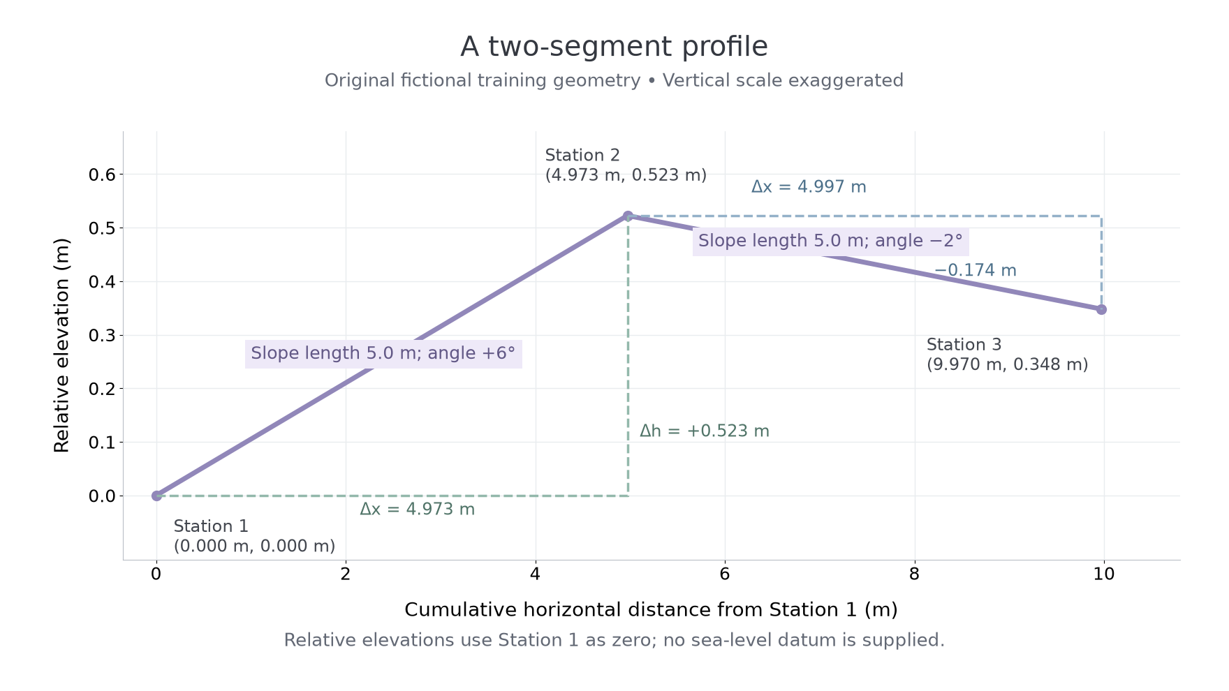
Original fictional training profile. The vertical scale is exaggerated so the changes are visible; the dashed lines show calculated horizontal and vertical changes, not extra observed stations.

Sighting at unequal pole heights, non-vertical poles, tape sag or a clinometer zero error can introduce systematic error. Long intervals can miss a small feature. Different starting positions can make repeated profiles appear to show change when different surfaces were surveyed. Record the transect, starting reference, observation time and surveyed extent; on a beach, changing tide state may alter the accessible extent. Avoid surveying where conditions breach the approved plan.

Estimating river discharge

Discharge estimates combine a channel's cross-sectional area with its mean flow velocity at the same location and time.

A cross-section needs width and a justified set of depths that represent its shape. For unequal panels, estimate each panel area using its width and the mean of its two end depths, then sum the panels. Width multiplied by a representative mean depth is a simpler approximation; multiplying by the maximum depth usually overestimates the area. State the approximation and its limitations.