Appendix 1 2(c), 2(d)(i) - Graphs, scales and distributions

Matching data to graphs

A graph should make the question's pattern visible while respecting the data type. Categories such as land uses suit a bar chart with separated bars. Values changing through ordered time or distance can suit a line graph; joining points implies a meaningful sequence. Paired numerical measurements at the same sites suit a scatter graph, where each point preserves its pair. Do not join scatter points in an arbitrary order. A pie chart shows mutually exclusive parts of one whole; a 25% share occupies $25/100\times360=90\degree$. It is less useful for many similar small shares or comparing several distributions precisely.

Construct a graph by checking units, choosing a suitable axis range and interval, labelling axes, plotting accurately, then adding a key and source/date where needed. Unequal gaps in time must have proportional horizontal spacing. Report missing values; do not convert them to zero. A line across a missing observation is an interpolation assumption. Dual axes may make unrelated series appear to move together: compare actual units and scale choices before inferring a relationship.

On a linear scale, equal spaces represent equal additions. A vertical axis with ticks 0, 20, 40 and 60 has a constant interval of 20. Bar charts normally need a zero baseline because bar lengths encode magnitude. If a line graph uses a shortened axis to reveal small changes, label it clearly and discuss absolute change: a rise from 98 to 102 is about 4.1%, even if it fills most of the plotting area. Never let the display's visual slope stand in for a calculated rate.

Reading logarithmic scales

A logarithmic scale gives equal space to equal ratios, which helps display values spanning several orders of magnitude. On a base-10 log scale, 1, 10, 100 and 1,000 are equally spaced because each value is ten times the previous one. The gap from 10 to 100 is an addition of 90, while the gap from 100 to 1,000 is an addition of 900: equal visual gaps do not mean equal absolute changes.

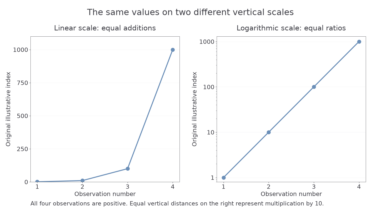
The values 1, 10, 100 and 1000 on linear and logarithmic vertical scales.

The original illustrative index rises by a factor of ten between each observation. Its log-scale line is straight because each equal horizontal step corresponds to the same multiplicative change. Its linear-scale line becomes much steeper because the absolute additions increase. Both displays are accurate, but emphasise different features.

To construct a log display, keep the original values and use a logarithmic axis; do not accidentally log the data and also use a log axis. Alternatively, plot transformed values on a linear axis and label it explicitly, such as $\log_{10}(x)$. An original value of 100 then has transformed value 2. The midpoint in log space between 10 and 100 is $\sqrt{10\times100}\approx31.6$, not 55. Ordinary logarithms cannot display zero or negative values. Do not quietly discard them or replace zero with one; explain the method or choose a suitable different display.

A log axis can make a huge absolute inequality look visually compact, while revealing relative differences that a linear scale hides. Read both axes and calculate the quantity that answers the question.

Transects and kite diagrams

A kite diagram shows how the abundance of several features changes along the same ordered transect. Each species or category has its own baseline. Width on both sides of that baseline is proportional to the recorded value; distance along the transect remains to scale.

The following percentage cover values are original illustrative observations from equal-sized quadrats. Species cover can overlap, so the two rows need not sum to 100% at each site.