6.7 - Land use, oceans and linked water-carbon risks

Land cover links carbon, water and soil

Changing vegetation alters both the amount of carbon stored on land and the pathways taken by rainfall.

Growing demand for food, timber, fuel and infrastructure encourages clearing, cultivation and extraction. When forest is burned, carbon in biomass enters the atmosphere rapidly; decomposition releases more after clearance. Removal also reduces future uptake by photosynthesis. Roots, litter and soil can store substantial carbon, so counting trunks alone misses part of the change. Harvested wood may retain carbon for a time, but its fate and the timescale must be considered.

An intact canopy intercepts rainfall and returns some water to the atmosphere through evaporation and transpiration. Roots and organic matter support infiltration; litter protects soil from raindrop impact. Clearing and compacting land can reduce infiltration, increase rapid overland flow and raise erosion and sediment loads. Losing topsoil reduces fertility, water retention and soil-carbon storage. However, reduced evapotranspiration can initially increase local water yield where rainfall stays similar; this does not contradict the possibility of lower regional rainfall when extensive forest loss reduces moisture recycling. Scale and timescale change the conclusion.

Afforestation establishes forest on previously non-forest land; reforestation re-establishes forest after loss. Growth can increase biomass carbon and protect soil, but species, age, management and former land cover matter. Planting on drained carbon-rich peat may release more soil carbon than new trees store. Water-demanding plantations can reduce local streamflow. Converting grassland to cropland can disturb roots and soil through ploughing, accelerate decomposition and erosion, and expose soil between crops; soil-conserving practices can moderate these effects.

Regional trends contrast. The FAO Global Forest Resources Assessment 2020 records net forest-area loss in Africa and South America during 2010–2020 and net gains in Asia, including a large gain in China. These regional totals combine different processes and do not prove that new plantations replace the biodiversity or carbon of old forests. Brazil's INPE November 2024 PRODES announcement estimated 6,288 km² of deforestation in the Legal Amazon for the 2024 monitoring year, 30.6% below 2023. A falling rate of loss still means forest is being lost; it is not a rise in total forest area.

Measuring land-cover change with GIS

GIS can locate changes between dates, but a credible calculation needs comparable classifications, image coverage and spatial units.

A geographical information system (GIS) combines spatially referenced layers so that location, attributes and change can be analysed together. For deforestation, use satellite imagery or a documented classified product such as INPE's PRODES, whose TerraBrasilis portal provides spatial downloads. A rigorous workflow is to define a study boundary, record dates and resolution, use a suitable common coordinate system, align the layers and apply the same land-cover definitions. Select comparable seasons and check cloud/shadow coverage; otherwise apparent change may be vegetation seasonality or missing observations.

Overlay the two classifications. Record forest→non-forest loss separately from non-forest→forest gain, and unchanged forest separately from both. A transition matrix counts each starting class against each ending class; net change subtracts gains and losses, whereas gross loss counts loss alone. For equal-area raster cells, area equals cell count multiplied by cell area. For latitude–longitude cells, do not assume equal area: use an appropriate equal-area projection or calculate areas correctly.

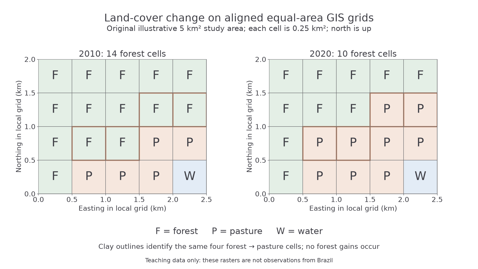
Original illustrative GIS rasters for the same 5 km² study area. Each cell is 0.5 km × 0.5 km = 0.25 km². F means forest, P pasture and W water; north is upwards. The outlined cells change from forest to pasture. These are not observations from Brazil.

The first raster has 14 forest cells and the second has 10. Four cells change from forest to pasture, with no gains, so gross forest loss is $4\times0.25=1.00\,\mathrm{km^2}$. Initial forest area is $14\times0.25=3.50\,\mathrm{km^2}$. Percentage loss relative to initial forest is $1.00/3.50\times100=28.6\%$, to one decimal place. Using the whole 5 km² map as the denominator would instead calculate the share of the study area that lost forest, 20%; it answers a different question.

A map shows where loss is clustered, so it can be compared with roads, rivers or protected-area boundaries. Such association can generate an explanation but does not prove a cause. Validate classification against independent high-resolution imagery or field evidence where available and ethical; report confusion between classes and the spatial distribution of unobserved cells. A small pixel can reveal a clearing but cannot measure all below-ground carbon, forest degradation or people's reasons for clearing. Written interpretation here checks analysis; practical GIS production remains a skill to perform.