5.3 - Water budgets, regimes and hydrographs
Learn to follow seasonal water storage, compare annual river regimes and explain the timing and size of a river's response to a storm using complete, labelled datasets.
A seasonal soil-water budget
A monthly water budget explains how rainfall and evaporative demand change soil-water availability through the year.
Potential evapotranspiration, or PET, is the water that could be lost if sufficient water were available. Actual evapotranspiration, or AET, is what is really lost. AET can match PET when precipitation and accessible stored water meet demand, but falls below it when water becomes limiting. The difference between them is a moisture deficit. A month with initially causes soil-water utilisation; it does not necessarily produce an immediate AET deficit.
For the simple soil-store model below:
After AET, the remaining water recharges soil up to its capacity. Any excess is surplus available for drainage. The monthly balance is , all in millimetres. This model omits capillary supply from deeper groundwater and assumes no other inputs.
This original illustrative temperate dataset has a soil capacity of 100 mm and starts January with 100 mm stored. Each month below is a monthly total; it is not a daily rate or an observed weather station record.
| Month | P, mm | PET, mm | End-of-month soil store, mm |
|---|---|---|---|
| Jan | 80 | 10 | 100 |
| Feb | 65 | 15 | 100 |
| Mar | 65 | 30 | 100 |
| Apr | 55 | 45 | 100 |
| May | 55 | 75 | 80 |
| Jun | 60 | 100 | 40 |
| Jul | 65 | 110 | 0 |
| Aug | 70 | 95 | 0 |
| Sep | 75 | 55 | 20 |
| Oct | 85 | 35 | 70 |
| Nov | 90 | 20 | 100 |
| Dec | 85 | 10 | 100 |
January has 70 mm of surplus because the store is already full. May uses 20 mm from storage, so AET is still 75 mm. July begins with 40 mm stored and receives 65 mm; only 105 mm is available against 110 mm of PET, giving a 5 mm deficit. August has no stored water, so AET is 70 mm and the deficit is 25 mm. September and October recharge soil without surplus. November supplies 70 mm after PET: 30 mm fills the store and 40 mm becomes surplus.
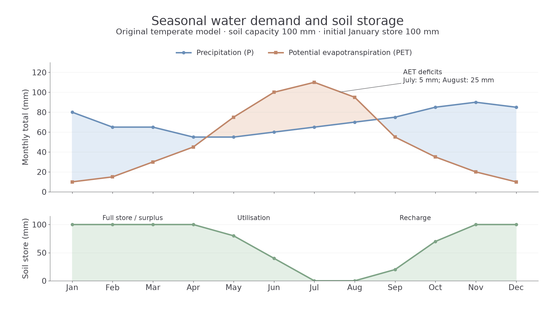
Seasonal water demand and storage in an original temperate model.
To construct this graph, put equally spaced months on the horizontal axis and use the same millimetre scale for P and PET. Plot both series, include a key and distinguish them from the separate storage series. Show utilisation, recharge and surplus only after calculating the store. Do not label every area where PET exceeds P as an AET deficit: stored soil water can meet some of the shortfall. Here annual P is 850 mm, PET is 600 mm and AET is 570 mm. Annual surplus is 280 mm and annual storage change is zero, so .
Budgets in contrasting climates
Climate controls the timing of water inputs and evaporative demand, so equal annual rainfall totals can produce different seasonal availability.
In a humid tropical rainforest climate, high temperatures maintain evaporative demand throughout the year. High precipitation can exceed that demand for much of the year, promoting soil recharge, drainage and river flow. A tropical climate with a pronounced dry season can still experience soil-water depletion despite a high annual rainfall total. Rainfall concentrated into a few months cannot automatically meet demand in later dry months without accessible storage.
In a temperate climate like the original model above, winter demand is low, so soil stores fill and surplus can drain to streams and aquifers. Summer demand rises with temperature and available energy; vegetation uses stored soil water and may become water stressed. The annual P–PET difference alone does not locate the period of shortage. Soil capacity, rooting depth, initial moisture and rainfall timing determine whether AET can meet PET.
In a polar or very cold basin, annual precipitation and evaporative demand can both be low. Winter precipitation is held as snow and soil water may be frozen, so a positive annual atmospheric balance does not mean water is immediately available to roots or rivers. Thaw produces a seasonal pulse. Frozen ground can restrict infiltration, increasing surface transfer; the result depends on thaw depth and local permeability. Polar water supply is limited by physical access and timing as well as volume.
For comparison, three original illustrative annual climate summaries are humid tropical P 2,100 mm/PET 1,500 mm, temperate P 850 mm/PET 600 mm and cold polar P 250 mm/PET 120 mm. Their P–PET values are +600, +250 and +130 mm. These differences describe climatic potential, not measured runoff. PET is demand, while the actual mass balance needs AET, storage change and all relevant transfers. A positive annual difference can coexist with a dry-season or frozen-season shortage.
Comparing annual river regimes
A river regime shows how average discharge varies through the months of a year, rather than how one storm develops over hours.
Discharge is the volume passing a cross-section per unit time, commonly . A regime normally uses monthly means calculated over a stated multi-year period at a named gauge. Gauge location, basin area, averaging years and reservoir operations matter. Do not compare two stations as though they represented equal catchments, or use a single exceptional year as a long-term regime.
The table is an original illustrative comparison of characteristic seasonal patterns. Its values are dimensionless monthly discharge divided by each series' own annual mean; each series has mean 1.00. These are not observed Yukon, Amazon or Indus gauge values and cannot establish which real river carries the greatest volume.
| Month | Yukon-type snowmelt | Amazon-type humid tropical | Indus-type melt/monsoon |
|---|---|---|---|
| Jan | 0.20 | 0.85 | 0.35 |
| Feb | 0.20 | 0.95 | 0.35 |
| Mar | 0.20 | 1.05 | 0.45 |
| Apr | 0.30 | 1.20 | 0.65 |
| May | 1.50 | 1.35 | 0.90 |
| Jun | 3.00 | 1.35 | 1.30 |
| Jul | 2.00 | 1.20 | 2.00 |
| Aug | 1.60 | 1.00 | 2.10 |
| Sep | 1.30 | 0.80 | 1.50 |
| Oct | 0.80 | 0.70 | 1.00 |
| Nov | 0.50 | 0.75 | 0.75 |
| Dec | 0.40 | 0.80 | 0.65 |
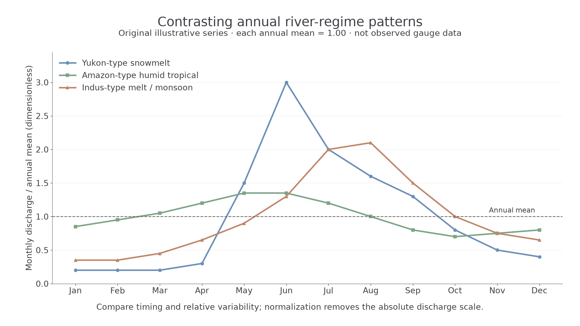
Original normalized regime patterns for comparing timing and variability.
Continue this lesson.
You’re previewing NovaLearn without an account. Create a free account to read the rest.
Create free account