2A.1 - Climate change through glacial time
Learn how repeated cold and warm phases produced changing ice cover, how different climate drivers operate over different timescales, and how climate reconstructions can be checked against landscape evidence.
Repeated cold and warm phases
The Pleistocene was a sequence of climatic changes rather than one uninterrupted period of expanding ice.
Glacial and interglacial
A glacial is a relatively cold interval when continental ice sheets and many mountain glaciers expand. An interglacial is a warmer interval between glacials, with reduced ice cover. Even an interglacial can retain large ice sheets.
The Pleistocene began about 2.58 million years ago and ended about 11,700 years ago. Early Pleistocene ice-volume changes were strongly paced by roughly 41,000-year cycles; later, particularly over the last approximately 800,000 years, major glacial cycles commonly lasted about 100,000 years. These are approximate patterns, not a clock that makes every cycle identical. A glacial itself may contain shorter cold stadials and warmer interstadials; these fluctuations are not the same scale as a full glacial–interglacial cycle.
| Interval or example | Approximate date | Meaning for ice cover |
|---|---|---|
| Start of Pleistocene | 2.58 million years ago | Beginning of the epoch containing repeated large Northern Hemisphere glaciations |
| Anglian glaciation in Britain | About 450,000 years ago | A particularly extensive British glaciation; its limit differs from the last glaciation |
| Last interglacial, called Ipswichian in Britain | About 129,000–116,000 years ago | Much smaller Northern Hemisphere ice sheets than in the following glacial |
| Last glacial, called Devensian in Britain | Broadly 115,000–11,700 years ago | Repeated advances and retreats; maximum ice extent varied between regions |
| Global Last Glacial Maximum | Broadly 26,500–19,000 years ago | Large land-ice volumes, rather than the beginning of the entire last glacial |
| Holocene | From about 11,700 years ago | Present interglacial, with Greenland and Antarctic ice sheets remaining |
Dates are rounded and regional boundaries are not all synchronous. British stages should not be treated as names for every region's ice history. Deglaciation also included reversals: the Younger Dryas, approximately 12,900–11,700 years ago, brought renewed cold conditions before the Holocene.
The specification uses Anthropocene to frame strong human effects on the Earth system, especially recent greenhouse-gas increases. It is widely used in that sense, but the proposal to make it a formal geological epoch was rejected in 2024. The formal present epoch remains the Holocene. This naming decision does not remove the evidence of human-caused climate change.
Orbital changes and summer snow survival
Ice sheets grow when enough winter snow survives successive summers, so summer conditions at high northern latitudes are especially important.
Milankovitch cycles alter the seasonal and latitudinal distribution of incoming solar radiation, or insolation. Eccentricity changes the shape of Earth's orbit, with an important cycle near 100,000 years. Obliquity changes axial tilt over about 41,000 years. Precession changes the orientation of the axis relative to Earth's orbital position, producing cycles around 19,000–23,000 years. They interact; eccentricity's direct effect on global annual energy is small, but it changes the strength of seasonal effects associated with precession.
For example, a configuration producing weaker northern high-latitude summers can reduce snowmelt. Snow surviving one summer provides the starting surface for the next winter's accumulation. An expanding bright snow and ice surface reflects more sunlight, reinforcing cooling. Ocean circulation, vegetation and greenhouse gases modify the response, so an orbital forcing is amplified into much larger changes in temperature and ice volume.
Orbit does not determine a single local glacier's behaviour by itself. Snowfall, topography and regional circulation decide where ice actually grows. Nor can slowly changing orbital conditions explain the rapid warming since industrialisation: their characteristic timescales are tens of thousands of years, whereas the recent change occurs over decades to centuries.
Orbital cycles pace long-term climate change by redistributing insolation. The survival of summer snow and climate feedbacks connect that redistribution to ice-sheet growth.
Solar, volcanic and atmospheric influences
Several drivers can change Earth's energy balance on timescales much shorter than an orbital cycle.
Solar output varies, including an approximately 11-year activity cycle. A sustained reduction in solar energy can contribute to cooling, but neither an individual sunspot count nor a coincidence with a cold episode proves the whole cause. The amplitude, duration and geographical response must match the proposed explanation.
Large explosive volcanic eruptions can inject sulphur dioxide into the stratosphere. Sulphate aerosols reflect some incoming sunlight, causing temporary surface cooling until they are removed, commonly over a few years. Ash is usually removed faster. Volcanoes also release carbon dioxide, but a short aerosol cooling effect is different from the long-lived greenhouse effect of carbon dioxide. Mount Pinatubo's 1991 eruption is an example of an event-scale influence; it does not explain repeated 100,000-year glacial cycles.
Changes in atmospheric composition affect outgoing longwave radiation. Carbon dioxide, methane and water vapour absorb and re-emit this radiation. More persistent greenhouse gases increase energy retained by the lower atmosphere and surface. During glacial cycles, changes in ocean carbon storage and other processes altered carbon dioxide and amplified temperature change. A driver and a feedback are different roles: an initial warming may release carbon dioxide, which then strengthens the warming.
In the Holocene, orbital redistribution continued while solar variation and eruptions contributed to shorter fluctuations. Since industrialisation, fossil-fuel burning and land-use change have raised greenhouse-gas concentrations. Increased water vapour in a warmer atmosphere then amplifies warming. Human influence explains the modern sustained warming far better than invoking an unspecified “natural cycle”. This conclusion depends on measured forcing and attribution, not simply on the Anthropocene label.
Comparing climate graphs and landforms
A reconstructed climate curve and a glacial landform record different things, so agreement must be tested rather than assumed.
Ice-core oxygen-isotope ratios provide a temperature-related proxy, while trapped gases record past atmospheric composition. Marine sediment oxygen isotopes reflect a combination of ice volume and ocean temperature. Each requires calibration and an age model. A proxy is evidence interpreted through a physical relationship; it is not a thermometer reading preserved without uncertainty.
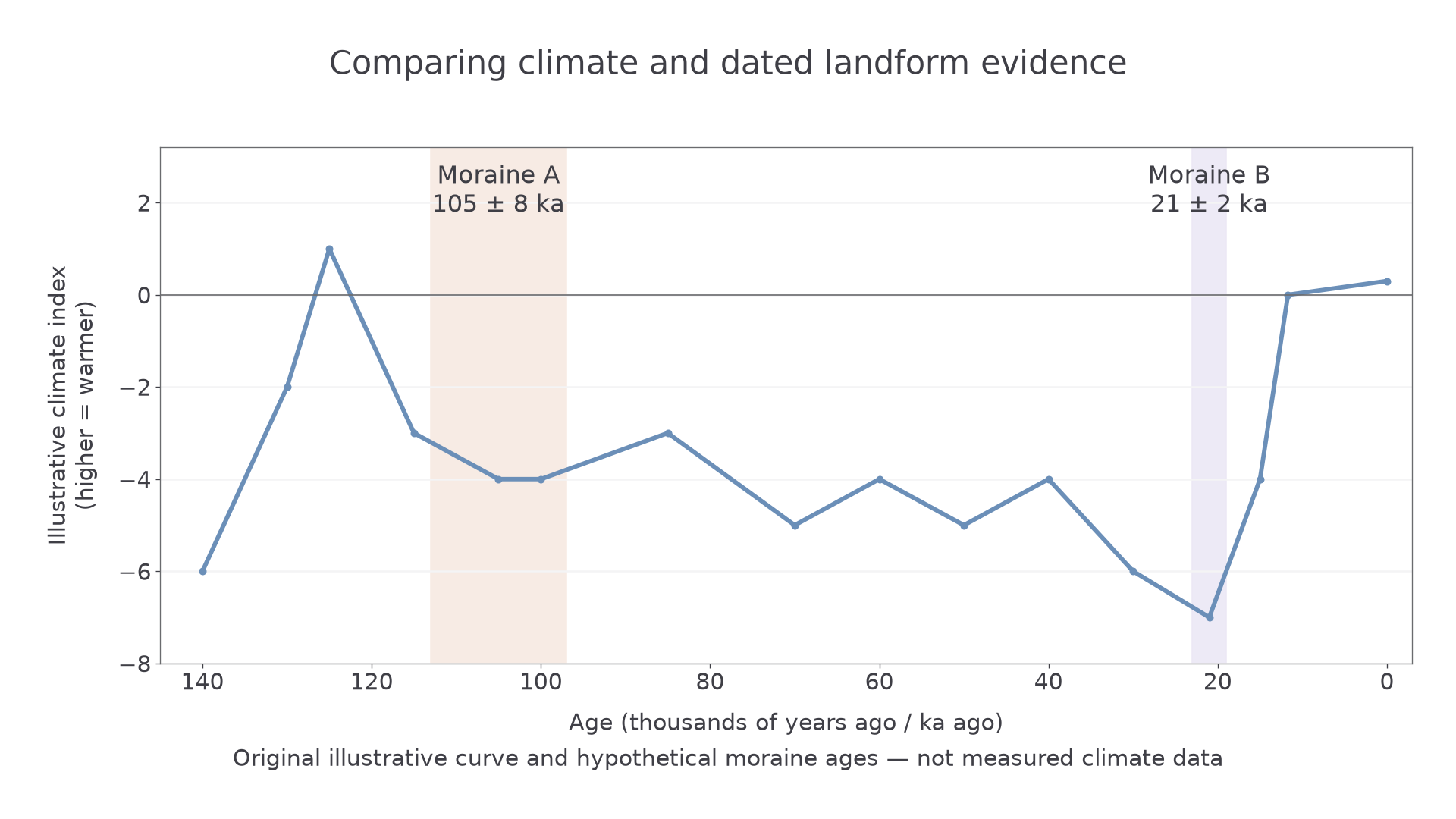
Original illustrative values and hypothetical moraine ages; this is a method demonstration, not an observed climate reconstruction. Higher index values represent warmer conditions.
Read the axes first: “ka ago” means thousands of years ago, with the older past at the left. Identify warm peaks and cold troughs, then compare the age range of a dated moraine with the climatic interval. In the example, moraine A at 105 ± 8 ka falls within the prolonged cooling after the warm peak; moraine B at 21 ± 2 ka coincides with a particularly cold interval. Neither match proves that temperature alone determined the local ice margin.
A moraine records an ice-margin position, often during a stillstand or readvance. It can survive after the glacier has disappeared. A glacial trough can be enlarged during several glaciations and therefore cannot be assigned the age of the nearest cold trough from its shape alone. Exposure dating, sediment relationships and several sites help distinguish events. Dating uncertainty, missing deposits, erosion by later ice and the lag between climate and ice response can all weaken an apparent match.
A defensible interpretation names the pattern, gives numerical or chronological evidence, explains the likely relationship, then states its limits. If a warm interval contains a preserved old moraine, that is not a contradiction: the moraine may be a relict from an earlier cold phase.