S6 - Scatter graphs, correlation and prediction
A scatter graph keeps two measurements from each case together. Learn to plot paired observations, recognise correlation, estimate a line of best fit and make predictions whose limits are clear.
Plotting paired observations
If people who practise longer tend to score more highly, does one extra hour guarantee a higher score? A scatter graph lets you examine that claim while keeping each person's hours and score together.
You already know
In coordinates , the horizontal value comes first. Use regular numerical scales with clear labels and units.
Bivariate data record two variables for each case. Each scatter point represents one case's pair. Unlike a time series, the points are usually different cases rather than successive readings of one case, so do not connect them in record order.
Worked example 1: keeping observations paired
Question. Plot practice hours and scores , with hours horizontally.
Plan. Label axes and plot each supplied pair without changing its pairing.
Why this step? Sorting the score column separately would give some people someone else's score.
Answer. Plot the six unjoined points on regular hours and score axes covering all values.
Check. Match each plotted point back to its original row, including the score fall between 3 and 4 hours.
The next example changes only the axis order. A coordinate's meaning follows the axis labels, not the order you happen to read a table.
Worked example 2: reversing the axes
Question. Plot the same observations with score horizontally and hours vertically.
Plan. Reverse each pair because the horizontal variable has changed.
Why this step? The 3-hour, score-5 person is still the same case, now at .
Answer. Plot those six unjoined points on score and hours axes.
Check. Reversing the coordinates again recovers every original pair.
For parcels with masses 2, 5 and 8 kg and respective postage costs £6, £10 and £13, a mass-horizontal plot uses . Label the units and choose regular scales, such as 1 kg and £2 per marked interval. A scatter axis need not start at zero, but a non-zero start must be clearly visible.
Watch out
Wrong: sort hours and scores separately before pairing the smallest with the smallest. This manufactures a pattern. Keep original rows together and use the stated horizontal variable first.
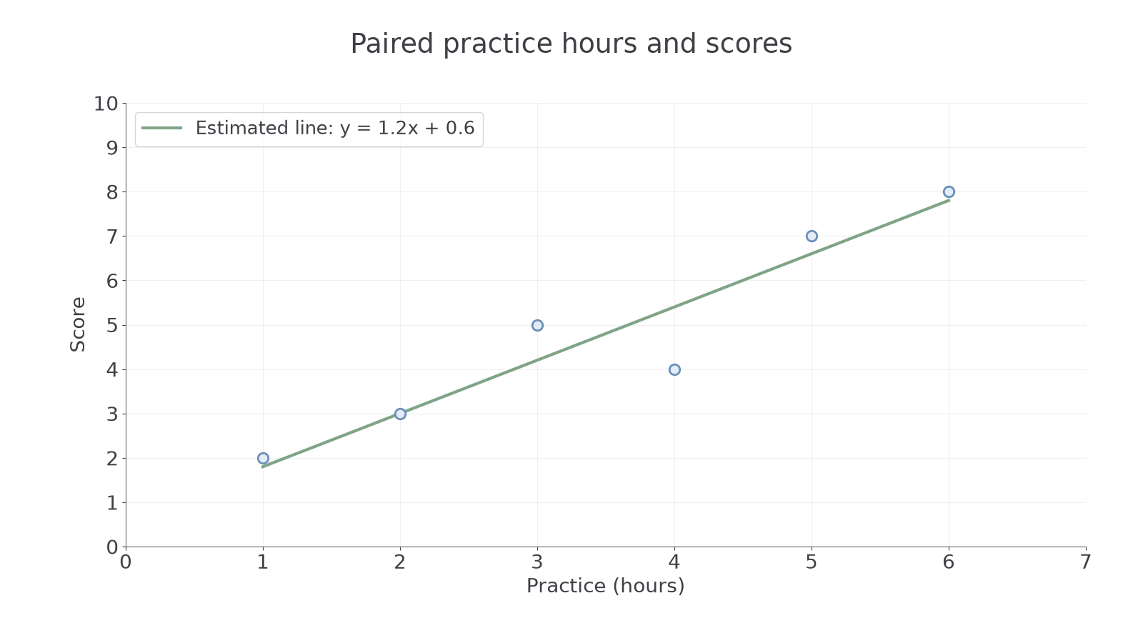
The graph below uses hours horizontally. Its straight line summarises the pattern; you will learn to judge that line in Part 3.
[DIAGRAM: asset_name: Paired practice and score data; asset_slug: 1ma1_m71_scatter; caption: Each point represents one observation; the estimated line summarises the association without joining every point.; description: Scatter graph of practice hours x and score y with points (1,2), (2,3), (3,5), (4,4), (5,7), (6,8), and an estimated straight line y equals 1.2x plus 0.6 over the observed interval.]
Use a new set of pairs, with the axis order made explicit.
Correlation and its causal limits
Correlation describes an overall association, rather than a rule that every next point must follow.
Correlation
With positive correlation, larger values of one variable tend to accompany larger values of the other. With negative correlation, larger values tend to accompany smaller values. No correlation means no clear overall association is evident in the graph.
A strong straight-line association has points close to an imagined straight line; a weaker one has more scatter. A strongly curved pattern is a relationship too, but a straight-line model may not describe it well. An unusual point may weaken the apparent pattern or suggest a case worth investigating.
The practice graph shows positive correlation even though the score drops from 5 to 4 as hours rise from 3 to 4. One local fall does not overturn the overall rising tendency. That is a useful surprise: positive correlation does not require every larger input to have a larger output.
Correlation does not establish causation. Larger households may buy more bread and more milk because household size affects both. Buying bread need not cause milk purchases. An observational graph alone cannot rule out a shared influence, reverse causation or other differences between groups.
Key idea
Describe what the cloud tends to do, then keep causal claims separate. “Higher practice hours tend to accompany higher scores” is supported by the plot; “one more hour must raise this person's score” is not.
A causal explanation needs evidence beyond a scatter pattern. The following check asks you to identify one plausible shared influence.
Estimating a line of best fit
An estimated line of best fit summarises a roughly straight pattern through the centre of a scatter cloud.
Continue this lesson.
You’re previewing NovaLearn without an account. Create a free account to read the rest.
Create free account