S3, S4 - Cumulative frequency, quartiles and box plots

How can you compare two groups without listing every measurement? S3 uses cumulative frequency to estimate positions in grouped data. S4 uses quartiles, box plots and spread to compare typical values and consistency, while keeping the limits of these summaries clear.

Accumulating frequencies and plotting boundaries (Higher)

Two delivery services can have the same typical time but different reliability. How can a picture show both the centre and the spread? Start by counting how many deliveries have finished by each time boundary.

You already know

A frequency table counts observations in classes. Grouped data hide individual measurements; values read inside a class are estimates rather than exact observations.

A cumulative frequency is the running total up to a stated value. If a class includes its upper boundary, its cumulative total counts all observations at or below that boundary. Plot the upper boundary, not the midpoint: each plotted total includes all earlier classes too.

Worked example 1: constructing a cumulative graph

Question. Times in minutes have classes $0<t\leq10$ , $10<t\leq20$ , $20<t\leq30$ , $30<t\leq40$ with frequencies 4, 10, 16 and 10. Construct a cumulative-frequency graph.

Plan. Add running totals, pair them with upper boundaries and plot.

\begin{aligned} \text{running totals}&=4,4+10,14+16,30+10 &&\text{accumulate counts}\\ &=4,14,30,40\\ \text{points}&=(0,0),(10,4),(20,14),(30,30),(40,40) &&\text{use class boundaries} \end{aligned}

Why include $(0,0)$ ? No time in this table is at or below the lower boundary, so it starts the cumulative graph.

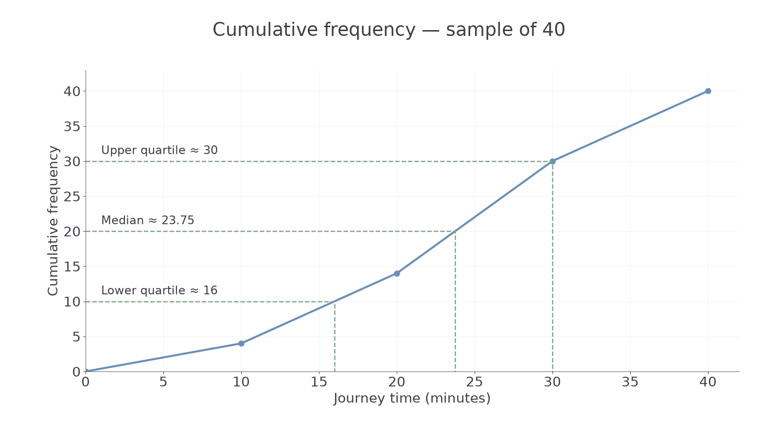
Answer. Plot on regular time and cumulative-frequency axes and join with a suitable increasing cumulative curve. Straight segments, as shown, model even distribution within classes.

Check. The graph never falls and ends at total frequency 40.

[DIAGRAM: asset_name: A cumulative journey-time distribution; asset_slug: 1ma1_m73_cumulative; caption: Running totals are plotted at upper class boundaries; the curve's final height is forty.; description: Cumulative frequency graph through (0,0), (10,4), (20,14), (30,30) and (40,40), with time in minutes horizontally and cumulative frequency vertically. Horizontal quartile levels at 10, 20 and 30 indicate readings near 16, 23.75 and 30 minutes.]
Running totals are plotted at upper class boundaries

The next example changes only the final class's upper boundary from 40 to 50 minutes. Frequency totals stay the same; the final horizontal gap changes.

Worked example 2: an unequal final class width

Question. Keep frequencies 4, 10, 16 and 10, with the last class now $30<t\leq50$ . Give the graph coordinates and count times over 10 and at most 30 minutes.

Plan. Keep running totals, update the last boundary and subtract cumulative counts for the requested interval.

\begin{aligned} \text{points}&=(0,0),(10,4),(20,14),(30,30),(50,40) &&\text{new final boundary}\\ \text{interval count}&=30-4=26 &&\text{exclude times at most 10} \end{aligned}

Why subtract? The count at 30 includes the four observations at or below 10, which the interval excludes.

Answer. Plot the coordinates with a final horizontal span of 20 minutes; the requested count is 26.

Check. $10+16=26$ , agreeing with the two complete class frequencies.

For unequal mass classes 0–5, 5–15 and 15–25 kg with frequencies 6, 9 and 5, cumulative points are $(0,0),(5,6),(15,15),(25,20)$ . The count over 5 and at most 25 kg is $20-6=14$ . At a supplied boundary the table fixes the count; between boundaries you estimate from the drawn graph.

Watch out

Wrong: plot the cumulative count 14 at midpoint 15 of the class 10–20. That count includes everything up to 20, so its point is $(20,14)$ . A midpoint belongs to a frequency polygon, not this construction.

Use upper boundaries in a new table.

Reading quartiles and interquartile range (Higher)

Quartiles locate quarter positions in an ordered distribution; their horizontal readings are measurements, not cumulative counts.

The lower quartile $Q_1$ has roughly a quarter of observations below it; the median has roughly half below it; the upper quartile $Q_3$ has roughly three quarters below it. For a grouped distribution of $n$ observations, use cumulative levels $n/4$ , $n/2$ and $3n/4$ . Move horizontally from each level to the graph, then down to the measurement axis. These level rules are not on the formula sheet: derive them from quarter and half proportions.

Interquartile range

\mathrm{IQR}=Q_3-Q_1

The interquartile range measures the spread of the middle half of the distribution, in the original measurement units.

Not on the formula sheet: learn it.

When the graph uses straight segments, a proportional width calculation gives the same reading as tracing along those segments. A suitable smooth cumulative curve may give nearby estimates.

Worked example 3: quartiles from a cumulative graph

Question. Estimate quartiles and IQR from the 40-journey straight-segment graph through $(0,0),(10,4),(20,14),(30,30),(40,40)$ .

Plan. Find the quarter-count levels, then estimate the corresponding times.

\begin{aligned} \text{levels}&=10,20,30 &&\text{quarters of 40}\\ Q_1&\approx10+\frac{10-4}{10}\times10=16\,\mathrm{min} &&\text{6 into a class of 10}\\ \text{median}&\approx20+\frac{20-14}{16}\times10=23.75\,\mathrm{min} &&\text{6 into a class of 16}\\ Q_3&\approx30\,\mathrm{min} &&\text{level 30 meets a boundary}\\ \mathrm{IQR}&\approx30-16=14\,\mathrm{min} &&\text{subtract time values} \end{aligned}

Why this step? Cumulative level 10 means ten observations, not a ten-minute lower quartile.

Answer. Estimated quartiles 16, 23.75 and 30 minutes; estimated IQR 14 minutes.

Check. They are ordered and lie within the plotted measurement range.

The next example doubles only the frequencies. This changes cumulative levels but leaves the distribution's proportions unchanged.

Worked example 4: a larger sample with the same proportions

Question. Frequencies in the same four classes are now 8, 20, 32 and 20. Estimate quartiles and IQR using straight segments.

Plan. Use quarters of the new total 80 and corresponding new cumulative counts.

\begin{aligned} \text{running totals}&=8,28,60,80 &&\text{twice the original totals}\\ \text{levels}&=20,40,60 &&\text{quarters of 80}\\ Q_1&\approx10+\frac{20-8}{20}\times10=16 &&\text{same fraction through class}\\ \text{median}&\approx20+\frac{40-28}{32}\times10=23.75 &&\text{same middle position proportion}\\ Q_3&\approx30,\quad\mathrm{IQR}\approx14 &&\text{read and subtract times} \end{aligned}

Why this step? Use equal cumulative proportions, not the same raw count level, when sample sizes change.

Answer. The same estimated quartiles and IQR, in minutes.

Check. $12/20=6/10$ and $12/32=6/16$ ; the within-class fractions are unchanged.

For small ordered lists, follow a task's stated quartile convention. One common instruction is to take medians of the lower and upper halves.

Worked example 5: quartiles of a supplied ordered list

Question. Use medians of halves for $2,3,4,5,7,8,9,10$ . Find median, quartiles and IQR.

Plan. Split the eight-value list into two four-value halves.

\begin{aligned} \text{median}&=(5+7)\div2=6 &&\text{middle of the full list}\\ Q_1&=(3+4)\div2=3.5 &&\text{middle of }2,3,4,5\\ Q_3&=(8+9)\div2=8.5 &&\text{middle of }7,8,9,10\\ \mathrm{IQR}&=8.5-3.5=5 &&\text{quartile difference} \end{aligned}

Why this step? The task specifies a convention for the individual list; grouped graphs instead use cumulative quarter positions.

Answer. Median 6, quartiles 3.5 and 8.5, IQR 5.

Check. The quartiles straddle the median and the IQR is smaller than the full range 8.

The overall range uses observed minimum and maximum. Grouped class endpoints do not necessarily reveal those exact extremes.

Watch out

Wrong: “For 80 measurements, IQR $=60-20=40$ .” Those are cumulative positions. Read $Q_1$ and $Q_3$ on the measurement axis, then subtract their values.

Now use supplied quartile readings for a different distribution.

Continue this lesson.

You’re previewing NovaLearn without an account. Create a free account to read the rest.

Create free account

Last Accessed

Papers 1, 2 and 3

S3, S4 - Cumulative frequency, quartiles and box plots

Accumulating frequencies and plotting boundaries (Higher)

Reading quartiles and interquartile range (Higher)

Continue this lesson.

Learn faster with Nova