S3 - Histograms and frequency density

A histogram uses area to represent frequency, so unequal class widths need more than a comparison of heights. Learn to construct and read histograms, recover frequencies and scales, and estimate a median or probability from grouped data with the assumptions stated.

Why area represents frequency (Higher)

Can a lower histogram bar contain more journeys than a taller one? Consider 30 journeys spread across 20 minutes, compared with 20 journeys spread across 10 minutes. The wider interval needs more horizontal space.

You already know

A rectangle's area is width multiplied by height. Frequency is a count, and a numerical class width is its upper boundary minus its lower boundary.

A histogram bar covers a numerical interval. Its area represents the frequency, so its height must be frequency divided by width. Equal widths allow height comparisons; unequal widths require area comparisons.

Frequency density

\text{frequency density}=\frac{\text{frequency}}{\text{class width}} \qquad \text{frequency}=\text{class width}\times\text{frequency density}

Class widths must be positive. Not on the formula sheet: learn it.

Put boundaries on a regular horizontal numerical scale, label the variable and units, then draw each bar across its complete interval. Adjacent classes touch. Label the vertical axis frequency density when plotting these heights.

Worked example 1: unequal class widths

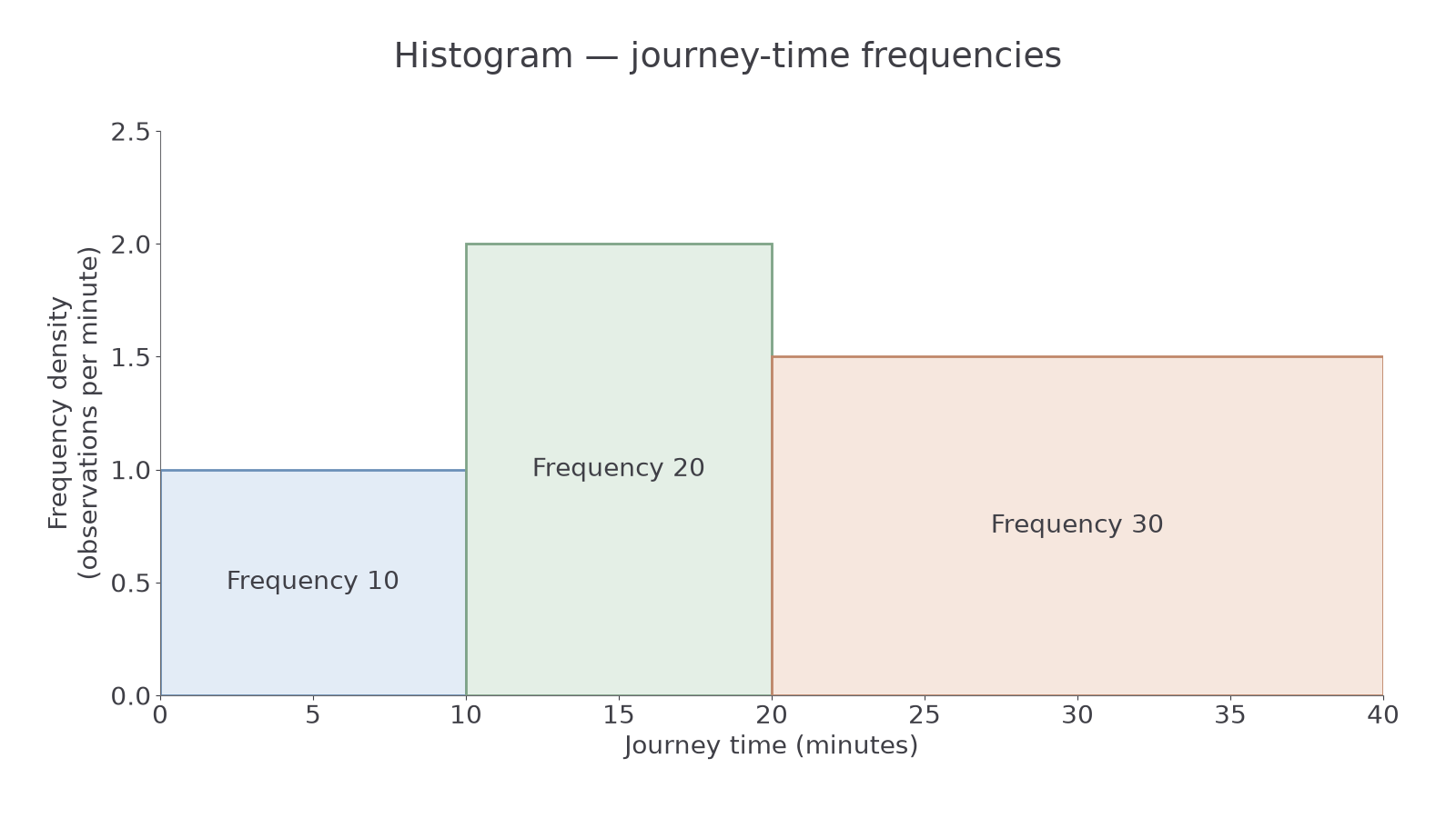
Question. Draw a histogram for journey times: $0<t\leq10$ , frequency 10; $10<t\leq20$ , frequency 20; $20<t\leq40$ , frequency 30, in minutes.

Plan. Calculate widths, divide for heights and check areas.

\begin{aligned} \text{widths}&=10,10,20 &&\text{subtract the boundaries}\\ \text{densities}&=10\div10,20\div10,30\div20 &&\text{frequency divided by width}\\ &=1,2,1.5 &&\text{required bar heights} \end{aligned}

Why this step? The last class spans twice as many minutes, so frequency 30 does not mean height 30.

Answer. Draw adjacent bars at heights 1, 2 and 1.5 over the stated intervals.

Check. Areas are $10\times1=10$ , $10\times2=20$ , $20\times1.5=30$ . The lowest concentration need not mean the fewest observations.

[DIAGRAM: asset_name: Unequal class widths in a histogram; asset_slug: 1ma1_m72_histogram; caption: Frequency is bar area: the wider final class contains thirty journeys despite its lower density than the middle class.; description: Histogram with time boundaries 0, 10, 20 and 40 minutes and frequency densities 1, 2 and 1.5, respectively; the bars have frequencies 10, 20 and 30, with labelled time and density axes.]
Frequency is bar area: the wider final class contains thirty journeys despite its lower density than the middle class.

The next example changes only the final class's upper boundary, from 40 to 30 minutes, keeping all three frequencies.

Worked example 2: narrowing a class

Question. Keep frequencies 10, 20 and 30, but use classes $0<t\leq10$ , $10<t\leq20$ , $20<t\leq30$ . Find the histogram heights.

Plan. Recalculate the changed width before finding density.

\begin{aligned} \text{widths}&=10,10,10 &&\text{all classes now equal}\\ \text{densities}&=1,2,30\div10=3 &&\text{same frequencies, new final width} \end{aligned}

Why this step? Halving the final width doubles its height to keep the same area.

Answer. Heights 1, 2 and 3.

Check. The final area remains $10\times3=30$ , so all frequencies are unchanged.

This gives a useful fact: two classes can have equal frequency but very different heights. Frequency 30 in widths 5 and 20 gives heights 6 and 1.5; the wider bar is one quarter as tall.

Grouped discrete data can also have defined boundaries. Integer scores 0–4 and 5–9 can use boundaries $-0.5$ to 4.5 and 4.5 to 9.5, each width 5. The half-unit boundaries separate neighbouring possible whole-number scores; they are not extra observed scores.

Watch out

Wrong: “The middle bar has most journeys because it is tallest.” In the original histogram its area is 20, while the wider final bar's area is 30. Compare width times density, not height alone.

Use a new class and retain the area reasoning.

Recovering frequencies and scales (Higher)

Multiply width by density to recover a frequency; when a vertical scale is unnumbered, use one known frequency to calibrate areas.

Worked example 3: recovering a frequency

Question. A bar spans 20 to 35 and has frequency density 2.4. Find its frequency.

Plan. Find the interval width, then its area.

\begin{aligned} \text{width}&=35-20=15 &&\text{use both boundaries}\\ \text{frequency}&=15\times2.4=36 &&\text{area gives count} \end{aligned}

Why this step? The upper boundary 35 is not the bar's width.

Answer. 36 observations.

Check. $36\div15=2.4$ , recovering the density.

The next example changes only the height, from 2.4 to 3.2.

Worked example 4: changing the density

Question. The same 20-to-35 class has density 3.2. Find its frequency.

Plan. Keep the width and update the area.

\begin{aligned} \text{width}&=35-20=15 &&\text{interval unchanged}\\ \text{frequency}&=15\times3.2=48 &&\text{new bar area} \end{aligned}

Why this step? With width fixed, changing height scales frequency in the same proportion.

Answer. 48 observations.

Check. $48\div36=3.2\div2.4=4/3$ .

Rearranging the same result also finds a missing width: $36\div2.4=15$ ; or a missing density: $36\div15=2.4$ . These rearrangements are not on the formula sheet: derive them from frequency density.

Worked example 5: calibrating an unnumbered scale

Question. On common regular scales, bar A has plotted width 4, height 3 and frequency 24. Bar B has plotted width 6 and height 5. Find B's frequency.

Plan. Find the common frequency-per-plotted-area factor.

\begin{aligned} \text{area A}&=4\times3=12 &&\text{measure plotted area}\\ \text{factor}&=24\div12=2 &&\text{observations per area unit}\\ \text{area B}&=6\times5=30 &&\text{same plotted scales}\\ \text{frequency B}&=30\times2=60 &&\text{apply the common factor} \end{aligned}

Why this step? An unnumbered height is not automatically the actual density; the known bar fixes the scale.

Answer. 60 observations.

Check. B's area is $30/12=2.5$ times A's, and $60/24=2.5$ .

Add class frequencies to find the total. If a total is known, subtract known class frequencies to find a missing one before converting it to density. Counting grid squares measures area; it is the same method, provided both bars use common regular scales.

Watch out

Wrong: “B is $5/3$ times as high, so its frequency is $24\times5/3=40$ .” Width also changed. Use the area ratio $(6\times5)/(4\times3)$ , giving frequency 60.

Apply the same calibration to new plotted dimensions.

Estimating a median from a histogram (Higher)

A median splits the distribution in half, so find the horizontal value with half the total frequency area to its left.

You already know

The median describes the middle of ordered data. Histogram areas recover class frequencies, but grouping hides the individual observations within each class.

First calculate every class frequency as width times density. Add them to obtain $n$ , then target cumulative frequency $n/2$ . Running totals locate the median class. Subtract the frequency before that class to find how far into its frequency you must go.

Now assume observations are evenly distributed within the class. The required fraction of its frequency then occupies the same fraction of its width. Add that distance to the lower boundary. This interpolation is not on the formula sheet: derive it from frequency density and proportional widths. It gives an estimated median, not an exact observed median.

Worked example 6: a median inside a class

Question. A histogram has classes 0–10, 10–20 and 20–40 minutes, with densities 1, 3 and 1.5. Estimate the median, assuming even distribution within each class.

Plan. Recover areas, locate half the total, then take the required fraction of the median-class width.

\begin{aligned} \text{frequencies}&=10(1),10(3),20(1.5)=10,30,30 &&\text{bar areas}\\ n/2&=(10+30+30)\div2=35 &&\text{half of 70}\\ \text{running totals}&=10,40,70 &&\text{35 lies in 10–20}\\ \text{needed within class}&=35-10=25 &&\text{remove the earlier count}\\ \text{median estimate}&=10+\frac{25}{30}\times10=\frac{55}{3}\,\mathrm{min} &&\text{same fraction of width} \end{aligned}

Why this fraction? The median needs 25 of that class's 30 observations, so the even-distribution model uses $25/30$ of its width, not half the width automatically.

Answer. Estimated median $18.3$ minutes to one decimal place, under the even-distribution assumption.

Check. Area to the left is $10+(55/3-10)\times3=35$ , half of 70.

Continue this lesson.

You’re previewing NovaLearn without an account. Create a free account to read the rest.

Create free account

Last Accessed

Papers 1, 2 and 3

S3 - Histograms and frequency density

Why area represents frequency (Higher)

Recovering frequencies and scales (Higher)

Estimating a median from a histogram (Higher)

Continue this lesson.

Learn faster with Nova