A12, A14 - Cubic, reciprocal and real-context graphs

A12 helps you recognise cubic and reciprocal graphs. A14 uses graphs to explore unfamiliar rules and motion. You will calculate useful points, choose sensible joins and read distances, speeds and accelerations from labelled axes.

Cubic and reciprocal shapes

Can a graph get closer and closer to an axis without ever touching it? For $y=1/x$ , inputs 1, 2 and 4 give outputs 1, $\frac12$ and $\frac14$ . The output shrinks, but none of these points is on the horizontal axis.

You already know

A point $(x,y)$ records an input and its output. Use brackets when substituting a negative input into a power.

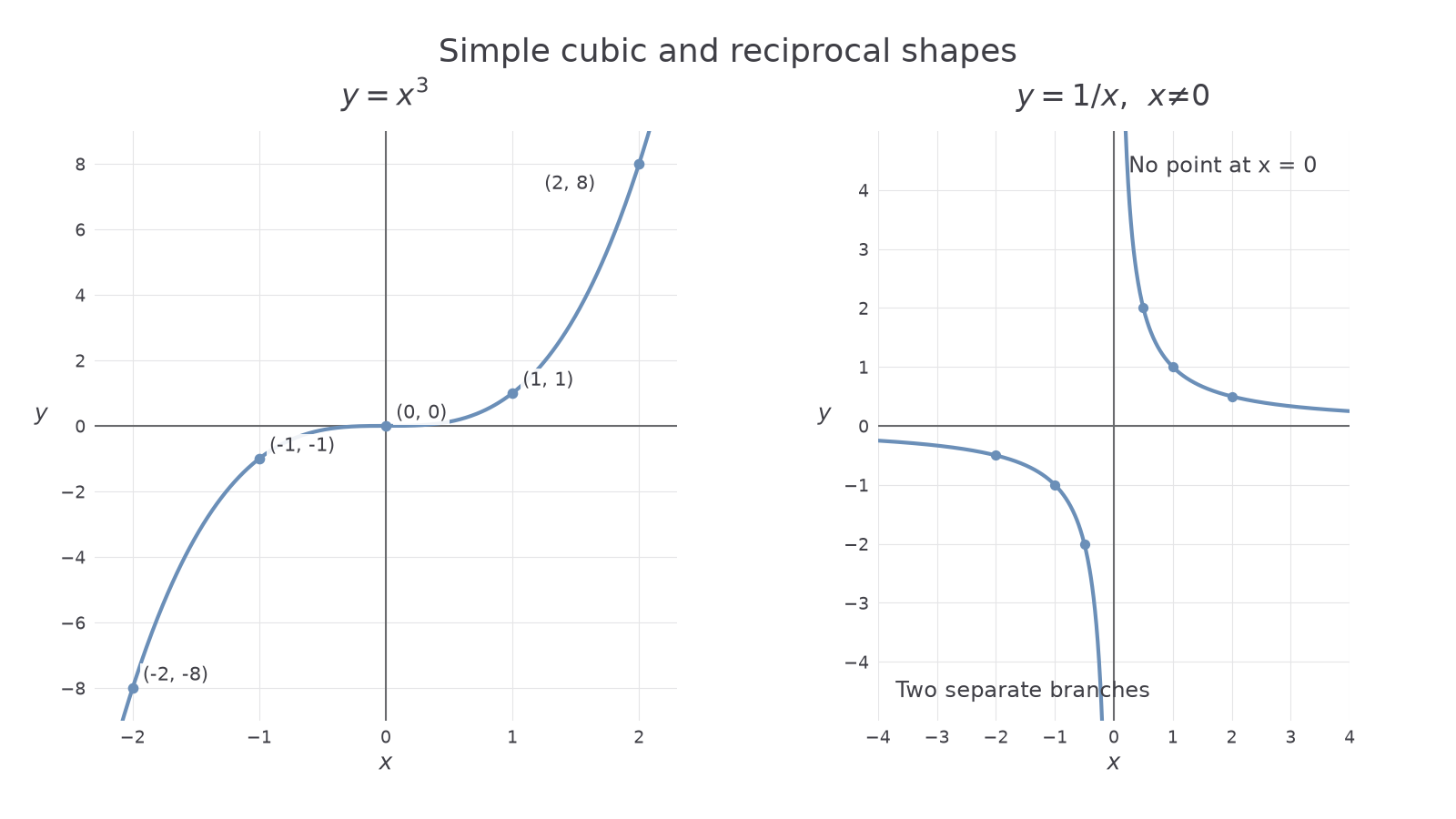
Compare two rules. The simple cubic $y=x^3$ passes through the origin and has a smooth S shape. Its outputs at $-2,-1,0,1,2$ are $-8,-1,0,1,8$ . It increases from bottom left to top right and flattens near the origin. For $y=-x^3$ , the output signs reverse and the graph decreases.

The reciprocal $y=1/x$ has two separate branches, with $x\ne0$ . A positive input gives a positive output; a negative input gives a negative output. Near zero, the magnitude becomes very large. Zero input is forbidden because division by zero is undefined.

Asymptote

An asymptote is a line that a graph approaches as an input approaches a limiting value or becomes very large in magnitude. For $y=1/x$ , the axes $x=0$ and $y=0$ are asymptotes. This reciprocal graph meets neither axis.

The cubic has a point at the origin; the reciprocal has no point there. That is a useful way to distinguish their shapes.

[DIAGRAM: asset_name: Simple cubic and reciprocal graphs; asset_slug: 1ma1_m25_cubic_reciprocal; caption: A cubic passes through the origin, while the reciprocal has two branches and excludes zero.; description: The left panel plots y equals x cubed with labelled table points from minus 2 to 2. The right panel plots y equals 1 over x on separate positive and negative input intervals, approaching both axes without crossing them.]
A cubic passes through the origin, while the reciprocal has two branches and excludes zero.

Worked example 1: compare two outputs

Question. Find the points with input 2 on $y=x^3$ and $y=1/x$ .

Plan. Substitute the same input into each rule.

\begin{aligned} y_{\text{cubic}}&=2^3=2\times2\times2=8 &&\text{cube the input}\\ y_{\text{reciprocal}}&=\frac12 &&\text{divide 1 by the input} \end{aligned}

Why this step? The rules use the input differently, so a similar-looking symbol does not mean a similar output.

Answer. The points are $(2,8)$ and $(2,\frac12)$ .

Check. The reciprocal output times its input is $\frac12\times2=1$ .

Change only the input sign next. Both graphs have a useful symmetry: opposite inputs give opposite outputs. A half-turn about the origin leaves either graph unchanged.

Worked example 2: negative inputs

Question. Find the points with input $-2$ on the same two graphs.

Plan. Include the negative sign in the whole input.

\begin{aligned} y_{\text{cubic}}&=(-2)^3=4(-2)=-8 &&\text{three negative factors}\\ y_{\text{reciprocal}}&=\frac1{-2}=-\frac12 &&\text{divide by a negative} \end{aligned}

Why this step? Cubing keeps the negative sign. Squaring the input instead would give the wrong graph.

Answer. The points are $(-2,-8)$ and $(-2,-\frac12)$ .

Check. Each is the half-turn image of the corresponding point in example 1.

For a paper sketch, calculate extra points at half-unit steps, plot them on labelled axes and draw smooth curves. Draw the reciprocal branches separately. For example, at $x=-0.5$ , its output is $-2$ ; at $x=0.5$ , its output is 2. A fraction with numerator 1 cannot equal zero for any permitted finite input.

Watch out

Writing $1/0=0$ is wrong: division by zero is undefined. Leave a gap at zero input and draw the reciprocal branches separately.

Check the signs carefully when the input is a negative fraction.

Plotting an unfamiliar rule in context

You do not need to recognise a rule's shape before you begin. Calculate a table, plot the points, then use the context to decide how to join them.

A water-depth model is $h=12/(t+2)$ , where $t$ is minutes and $h$ is centimetres, for $0\le t\le6$ .

$t$ , minutes	0	1	2	3	4	6
$h$ , centimetres	6	4	3	2.4	2	1.5

Put time on the horizontal axis and depth on the vertical axis. Choose regular scales covering the table. Depth changes continuously, so join the points with a smooth decreasing curve. The falls become smaller; a straight line between the first and last points would miss that behaviour.

Worked example 3: read a target depth

Question. Use the water model to estimate when the depth reaches $2.5\,\mathrm{cm}$ .

Plan. Read from height 2.5 across to the curve and down to time, then check using the rule.

\begin{aligned} \frac{12}{t+2}&=2.5 &&\text{set the target height}\\ t+2&=\frac{12}{2.5}=4.8 &&\text{find the denominator}\\ t&=2.8 &&\text{subtract 2} \end{aligned}

Why this step? A graph intersection means the rule's output equals the chosen target height.

Answer. The graph should give about 2.8 minutes.

Check. $12/(2.8+2)=2.5$ , and the time is inside the model's interval.

Now change only the target depth, from 2.5 to $2\,\mathrm{cm}$ . The same curve supplies the new answer.

Worked example 4: a second target on the same curve

Question. Estimate when the water depth reaches $2\,\mathrm{cm}$ .

Plan. Use the horizontal level 2 and check the time with the model.

\begin{aligned} \frac{12}{t+2}&=2 &&\text{set the new target}\\ t+2&=6 &&\text{divide 12 by 2}\\ t&=4 &&\text{subtract 2} \end{aligned}

Why this step? Changing the target changes the intersection, rather than changing the rule itself.

Answer. The depth reaches $2\,\mathrm{cm}$ after 4 minutes.

Check. The table contains $(4,2)$ , agreeing with the calculation.

On squared paper, construct this curve and add the two reading guides. If the curve between 2 and 3 minutes is unclear, calculate another point; $t=2.5$ gives $h=\frac83$ . Only the stated interval is supported. Being able to calculate the expression after 6 minutes does not establish that the real water continues to follow it.

Some inputs are discrete. For tickets costing £4 per person, $C=4n$ gives $(4,16)$ for four people. Plot whole-number inputs as separate points: 2.5 people is not an allowed purchase. The context decides whether intermediate inputs make sense.

Watch out

“Join the dots” is not a universal rule. Use a smooth curve for a continuous non-linear model, straight segments only when justified, and separate points for discrete counts.

Other unfamiliar rules work the same way. A cooling model $T=30/(t+1)+20$ , for $0\le t\le5$ , gives $30^\circ\mathrm{C}$ at 2 minutes. Its intersection with $T=26$ at $t=4$ means the modelled temperature is $26^\circ\mathrm{C}$ after 4 minutes.

Distance and displacement over time

Read the vertical label first. A height may mean total distance travelled, distance from a place, or signed displacement.

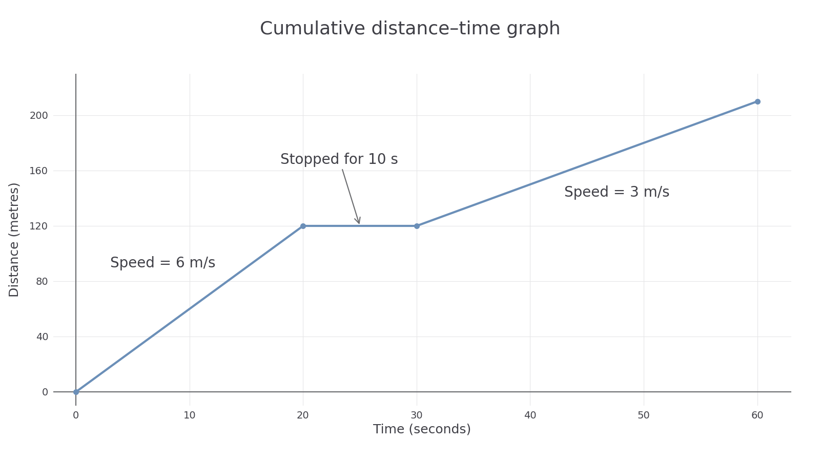
For cumulative distance, the height is the total distance travelled so far. A straight segment shows constant speed, and a horizontal segment shows a stop. Total distance cannot decrease: even walking back adds to it.

[DIAGRAM: asset_name: Cumulative distance-time graph; asset_slug: 1ma1_m25_distance_time; caption: A horizontal cumulative-distance segment means a stop, and straight-segment gradient gives speed.; description: The graph joins (0,0), (20,120), (30,120) and (60,210), showing a 10-second stop and travel speeds 6 and 3 metres per second. The horizontal axis is time in seconds and the vertical axis is cumulative distance in metres.]
A horizontal cumulative-distance segment means a stop, and straight-segment gradient gives speed.

Last Accessed

Papers 1, 2 and 3

A12, A14 - Cubic, reciprocal and real-context graphs

Cubic and reciprocal shapes

Plotting an unfamiliar rule in context

Distance and displacement over time

Continue this lesson.

Learn faster with Nova