P8 - Combined events and probability trees
P8 combines events through independent or dependent stages. You will build probability trees, multiply along complete paths and add successful alternatives, checking what the procedure assumes about replacement and independence. The final Higher part uses probability to find an unknown count.
Independent events and multiplication
Does putting a token back change your chance of drawing two blue tokens? It can: the procedure decides whether the second draw has the same chance as the first.
You already know
A complement has probability . Multiplying fractions finds a fraction of a fraction: half of one sixth is one twelfth.
A head on a fair coin and a six on an independent fair die has probability . In a list of twelve equally likely coin–die pairs, only one meets both conditions. Multiplication finds the share meeting the first condition and then the share of that group meeting the second.
Independent events
Two events are independent when knowing whether one occurs does not change the probability of the other. Separate fair coin tosses model this; draws without replacement usually do not, because the first draw changes the bag.
Independence must be stated or supported by the experiment. Merely naming two events does not establish it.
Independent combined events
If and are independent,
Not on the formula sheet: learn it.
“Both” asks for the intersection, not a choice between two alternatives.
Worked example 1: success in both games
Question. Two independent games have success probabilities and . Find the probability of success in both.
Plan. Multiply the two success probabilities.
Why this step? Of the share succeeding first, the same share succeeds second.
Answer. .
Check. is no larger than either individual success probability.
Change only the second required result from success to failure.
Worked example 2: success followed by failure
Question. For the same independent games, find the probability of success first and failure second.
Plan. Complement the second success probability before multiplying.
Why this step? The second factor must describe the required second result.
Answer. .
Check. : both second results recover all first successes.
When using a model, write the relevant independence assumption alongside the calculation if asked.
Watch out
Wrong: . Addition does not find the share meeting both conditions, and a probability cannot exceed one. Independence gives .
Change only the first success probability to , and make the modelling assumption precise.
Branches, paths and complete probability trees
A probability tree gives each stage its own split, so branch labels and whole-path probabilities stay separate.
Choose an order for the stages. Draw and label every first outcome, then repeat all second-stage outcomes under each first-stage outcome. Put each probability beside its own branch. Branches leaving one point must sum to one because they form exhaustive, mutually exclusive alternatives.
For two independent fair tosses, each split is , . The four paths each have probability , and their sum is one. A branch label describes only the next step from its starting point.
[DIAGRAM: asset_name: Independent pass and fail branches; asset_slug: 1ma1_m66_independent_tree; caption: Every local split sums to one; multiply the two branch labels to find each full path.; description: Two-stage probability tree for independent tests, first pass 0.6 and fail 0.4, second pass 0.7 and fail 0.3 under either first outcome. Leaves PP, PF, FP, FF have probabilities 0.42, 0.18, 0.28, 0.12.]
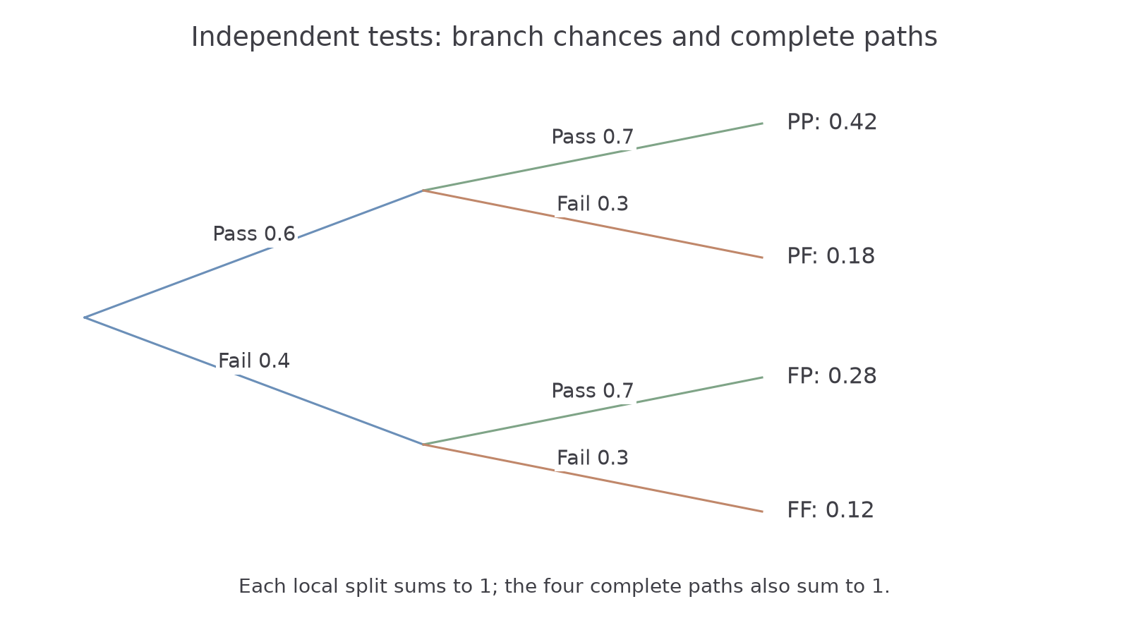
The path rule works by finding a proportion of a proportion. It is not on the formula sheet: learn to multiply the probabilities appropriate to each branch.
Worked example 3: building and checking a tree
Question. Independent tests have pass probabilities and . Complete their pass/fail tree and find the probability of passing both.
Plan. Complement both pass probabilities and multiply along each full path.
Why this step? Independence means both second splits use the same pair.
Answer. The completed tree is shown; passing both has probability .
Check. .
Keep the tree unchanged and change only the requested full path.
Worked example 4: a branch is not a leaf
Question. Find the probability of passing the first test and failing the second.
Plan. Follow the first pass branch and its second fail branch.
Why this step? The branch belongs only to people already at that second-stage split.
Answer. .
Check. , the first-pass chance.
Use local totals to catch a missing or misplaced branch label before calculating.
Watch out
Wrong: “Pass then fail has probability .” That is the second fail branch alone. The full path must also include the first pass: .
Keep the first test's probability fixed and change only the second pass probability to .
Sampling without replacement
Without replacement, the first result changes what remains, so update both the total and the relevant colour count before the next draw.
A bag with three red and two blue tokens has five tokens initially. After blue, four remain, including one blue and three red. After red, four remain, including two red and two blue. Draw a separate second split for each of those possible bags.
[DIAGRAM: asset_name: Two draws without replacement; asset_slug: 1ma1_m66_tree; caption: The first draw changes the second-stage probabilities; four complete paths remain.; description: Probability tree for a bag with three red and two blue tokens drawn twice without replacement. First branches red 3/5 and blue 2/5. After red branches red 2/4 and blue 2/4; after blue branches red 3/4 and blue 1/4. Leaves show RR 3/10, RB 3/10, BR 3/10 and BB 1/10.]
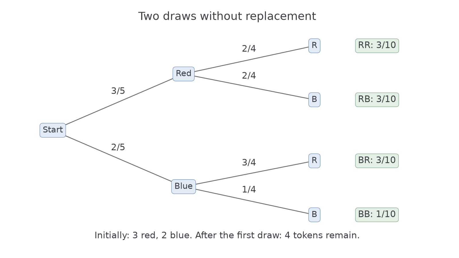
Keep multiplying along a path, using the second probability appropriate to its first result. This is the same path rule; independence is only needed to leave the second chance unchanged.
Worked example 5: two blue without replacement
Question. From this three-red, two-blue bag, draw two tokens uniformly without replacement. Find the probability of two blue.
Plan. Count the blues and total before each blue draw.
Why this step? The first blue is no longer available for the second draw.
Answer. .
Check. The four leaves in the tree sum to .
Change only the replacement rule: return the first token and mix before drawing again.
Worked example 6: two blue with replacement
Question. Find the probability of two blue from the same bag with replacement and mixing.
Plan. Restore the original blue fraction for the second draw.
Why this step? Replacement and mixing give the second draw the same distribution as the first.
Answer. .
Check. is greater than : returning a blue makes another blue more likely.
A second comparison uses six white and four black tokens. Two whites have probability with replacement, and without replacement. The procedure, not the word “random”, decides whether the fractions change.
Continue this lesson.
You’re previewing NovaLearn without an account. Create a free account to read the rest.
Create free account