A11, A12, A18 - Quadratic graphs and approximate roots

A quadratic graph's shape, roots and turning point reveal its behaviour (A11 and A12). You will plot and interpret these curves, find roots using factors, and estimate equation solutions from graph intersections (A18).

The shape and symmetry of quadratic graphs

A ball's height is modelled by $h=6t-t^2$ metres for $0\leq t\leq6$ seconds. When is it highest, how high does it go, and can it pass $4\,\mathrm{m}$ twice? A curved graph can show all three answers.

You already know

Substitute an input into the whole expression. In particular, $(-2)^2=4$ , because both negative factors are multiplied. A straight line is plotted using calculated coordinate pairs; a quadratic also starts with pairs, but needs a smooth curve.

For $y=x^2$ , inputs $0,1,2,3$ give outputs $0,1,4,9$ . Equal input steps give output changes $1,3,5$ , so the graph bends instead of rising at one constant rate.

Quadratic graph

A quadratic function has the form $y=ax^2+bx+c$ , with $a\ne0$ . Its graph is a parabola with a vertical line of symmetry and one turning point. It opens upwards if $a>0$ and downwards if $a<0$ . If $a=0$ , the rule is not quadratic.

The general form and shape rules are not on the formula sheet: learn them. The coefficient of the squared term decides the opening direction, rather than the sign of the constant.

Worked example 1: an upward-opening curve

Question. Plot $y=x^2-2x-3$ for $-2\leq x\leq4$ . State its symmetry line.

Plan. Calculate seven points, look for equal-height pairs and join the points smoothly.

\begin{aligned} x=-2 &: \ y=4+4-3=5 && \text{substitute the whole negative input} \\ x=-1 &: \ y=1+2-3=0 && \text{next input} \\ x=0 &: \ y=-3 && \text{vertical-axis crossing} \\ x=1 &: \ y=1-2-3=-4 && \text{central input} \\ x=2 &: \ y=4-4-3=-3 && \text{next input} \\ x=3 &: \ y=9-6-3=0 && \text{next input} \\ x=4 &: \ y=16-8-3=5 && \text{last input} \end{aligned}

Why use points on both sides? They show the turn and reveal matching heights, rather than only one arm of the curve.

Answer. Plot $(-2,5),(-1,0),(0,-3),(1,-4),(2,-3),(3,0),(4,5)$ and draw one smooth upward curve. Its symmetry line is $x=1$ .

Check. Inputs $-2,4$ , then $-1,3$ , then $0,2$ are equally far from $1$ and have matching outputs.

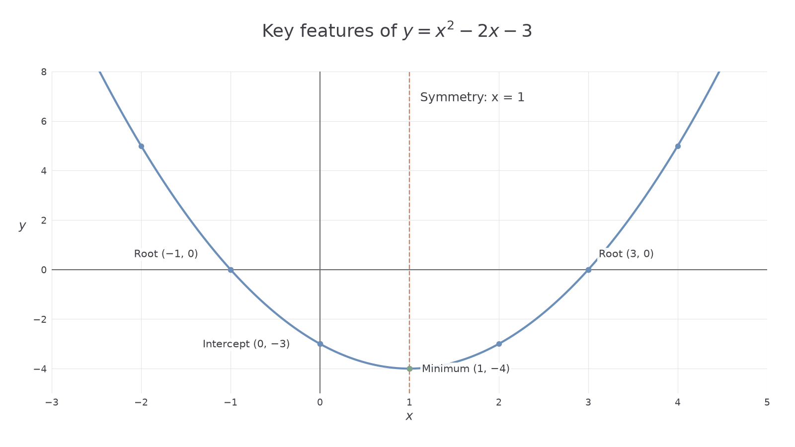
The plotted graph shows those points and the main features we will read in the next parts. On squared paper, choose regular labelled scales that include all seven points. Near the turn, draw a rounded curve through the points rather than a sharp corner.

[DIAGRAM: asset_name: A quadratic and its key features; asset_slug: 1ma1_m23_quadratic; caption: The roots, intercept and minimum identify the curve y equals x squared minus 2x minus 3.; description: Labelled axes plot the upward parabola, roots (-1,0) and (3,0), y-intercept (0,-3), minimum (1,-4) and dashed symmetry line x equals 1. The seven table points are shown.]

Change only the overall sign of the rule: every output becomes its opposite. The input positions and symmetry line stay fixed.

Worked example 2: reversing the opening direction

Question. Plot $y=-x^2+2x+3$ for $-2\leq x\leq4$ . State its symmetry line.

Plan. Substitute the same inputs, then join the new points smoothly.

\begin{aligned} x=-2 &: \ y=-4-4+3=-5 && \text{keep the minus outside the square} \\ x=-1 &: \ y=-1-2+3=0 && \text{next input} \\ x=0 &: \ y=3 && \text{vertical-axis crossing} \\ x=1 &: \ y=-1+2+3=4 && \text{central input} \\ x=2 &: \ y=-4+4+3=3 && \text{next input} \\ x=3 &: \ y=-9+6+3=0 && \text{next input} \\ x=4 &: \ y=-16+8+3=-5 && \text{last input} \end{aligned}

Why does the curve open downwards? The squared-term coefficient is negative; the table now rises to its central high point and falls again.

Answer. Plot $(-2,-5),(-1,0),(0,3),(1,4),(2,3),(3,0),(4,-5)$ , then draw a smooth downward curve. The symmetry line is still $x=1$ .

Check. Every output is the opposite of example 1's output, including the unchanged zeros.

A sketch need not reproduce a detailed grid, but must show the correct opening, axis crossings and important labelled points. For another downward curve, $y=9-x^2$ has outputs $5,9,5$ at inputs $-2,0,2$ , so its symmetry line is $x=0$ .

Watch out

Wrong: join quadratic points with ruler-made straight segments. That creates a zigzag. Right: draw one smooth curve through the calculated points, with a rounded turning point.

Change only the constant in the downward rule and use its shape and symmetry.

Roots and intercepts

A root is an input that produces output zero, so roots appear where the graph meets the horizontal axis.

Root and intercept

A root of $f(x)=0$ is a value of $x$ making the output zero. It gives an $x$ -intercept $(x,0)$ . The $y$ -intercept is where $x=0$ . A root is an input value; an intercept point has two coordinates.

Use the zero-product principle from factorised equations: if a product is zero, at least one complete factor is zero.

Worked example 3: two integer roots

Question. Find the roots and $y$ -intercept of $y=x^2-2x-3$ .

Plan. Factorise to find zero outputs, then set $x=0$ for the other axis crossing.

\begin{aligned} y&=(x-3)(x+1) && \text{factorise} \\ (x-3)(x+1)&=0 && \text{set the output to zero} \\ x-3=0&\quad\text{or}\quad x+1=0 && \text{zero-product principle} \\ x=3&\quad\text{or}\quad x=-1 && \text{solve both factors} \\ y\big|_{x=0}&=-3 && \text{vertical-axis crossing} \end{aligned}

Why set different variables to zero for the two axes? The horizontal axis has zero height; the vertical axis has zero horizontal position.

Answer. Roots $-1,3$ , with $x$ -intercepts $(-1,0),(3,0)$ ; $y$ -intercept $(0,-3)$ .

Check. The three crossings agree with the plotted curve, and both roots give zero in the original expression.

Change only the coefficient of $x$ in the second factor from one to two. Solve the complete factor, rather than just changing a constant's sign.

Worked example 4: a fractional root

Question. Find the roots and $y$ -intercept of $y=(x-3)(2x+1)$ .

Plan. Set each factor to zero, then substitute zero for the input.

\begin{aligned} x-3=0&\quad\text{or}\quad 2x+1=0 && \text{zero factors} \\ x=3&\quad\text{or}\quad 2x=-1 && \text{isolate the input terms} \\ x=3&\quad\text{or}\quad x=-\frac12 && \text{divide the second by two} \\ y\big|_{x=0}&=(-3)(1)=-3 && \text{find the vertical crossing} \end{aligned}

Why divide by two? The whole factor $2x+1$ must be zero; choosing $x=-1$ would leave it equal to $-1$ .

Answer. Roots $3,-1/2$ ; $y$ -intercept $(0,-3)$ .

Check. $2(-1/2)+1=0$ ; the other root makes the first factor zero.

The same process gives roots $-2,5$ and $y$ -intercept $(0,-10)$ for $y=(x+2)(x-5)$ . In general, $y=ax^2+bx+c$ meets the vertical axis at $(0,c)$ .

The “two” in a quadratic's degree does not promise two real roots. The graph of $y=x^2$ touches the axis at its repeated root $0$ ; it does not cross there. The graph of $y=x^2+2$ never reaches zero, so it has no real roots. By contrast, $y=x^2-1$ crosses at $-1$ and $1$ .

Watch out

Wrong: say the root from $2x+1$ is $-1$ . Right: solve $2x+1=0$ to get $-1/2$ . A coefficient on $x$ must be included.

The factorisation and zero-product rules are not on the formula sheet: learn them. Change the coefficient once more for your turn.

Turning points and extreme values

The turning point is where a quadratic changes between decreasing and increasing.

Maximum and minimum turning points

A minimum turning point is the lowest point of an upward-opening quadratic. A maximum turning point is the highest point of a downward-opening quadratic. Its vertical coordinate is the extreme output; its horizontal coordinate tells you where that output occurs.

Read a turning point by following its position to both labelled axes. Give a coordinate pair, then interpret each coordinate if the graph has a context.

Continue this lesson.

You’re previewing NovaLearn without an account. Create a free account to read the rest.

Create free account

Last Accessed

Papers 1, 2 and 3

A11, A12, A18 - Quadratic graphs and approximate roots

The shape and symmetry of quadratic graphs

Roots and intercepts

Turning points and extreme values

Continue this lesson.

Learn faster with Nova