4.4 - Normal approximations for rank tests
For samples beyond the supplied Wilcoxon tables, a normal approximation turns a rank sum into a familiar standardised statistic. Learn the two different mean–variance formulae, apply continuity corrections, and keep the tail consistent with the rank sum you chose.
Large-sample signed-rank distribution
If a signed-rank test has observations, can you use a table that ends at ? Use the large-sample distribution of a specified rank sum instead.
The original assumptions remain: independent random observations from a continuous population symmetric about its median, with no zero deviations or tied absolute ranks. For paired data, these are assumptions about the population of differences. An approximation does not remove them.
Under the null, rank contributes either or to the positive rank sum , with equal probabilities. Its mean contribution is , and its variance is . Independent signs give
Large-sample signed-rank model
For sufficiently large , either specified sum or is approximated under the null by
These mean and variance formulae are in the formula booklet. They apply to or , not to .
The second parameter is a variance: take its square root when standardising. Rank sums are integers, so include the observed integer's full interval: uses a normal boundary ; uses .
Worked example 1: an upper-tail approximation
Question. An independent random sample of observations satisfies the signed-rank assumptions. Relative to the proposed population median , the positive rank sum is . Use a normal approximation to test against , at .
Plan. A larger median gives a large positive rank sum, so approximate .
Under ,
The approximate upper-tail probability is , which is below .
Answer. Reject . There is sufficient evidence at the level that the population median exceeds .
Check. The total rank sum is , so . Its lower-tail boundary is , giving , the reflected tail with the same probability.
The half-unit correction is small on the plot, but it determines which whole-number outcomes the shaded area approximates.
[DIAGRAM: asset_name: Continuity correction for a signed-rank sum; asset_slug: cam9231-signed-rank-normal-tails; caption: The upper tail from P equals 219 starts at 218.5, while the equivalent lower tail from Q equals 81 ends at 81.5; description: Two exact normal density plots with mean 150 and standard deviation 35. The left plot shades values above 218.5 to approximate P at least 219. The right plot shades values below 81.5 to approximate Q at most 81. Each shows the mean, the half-unit boundary and an inset integer interval showing the relevant observed rank sum. Both shaded areas are approximately 0.0252.]
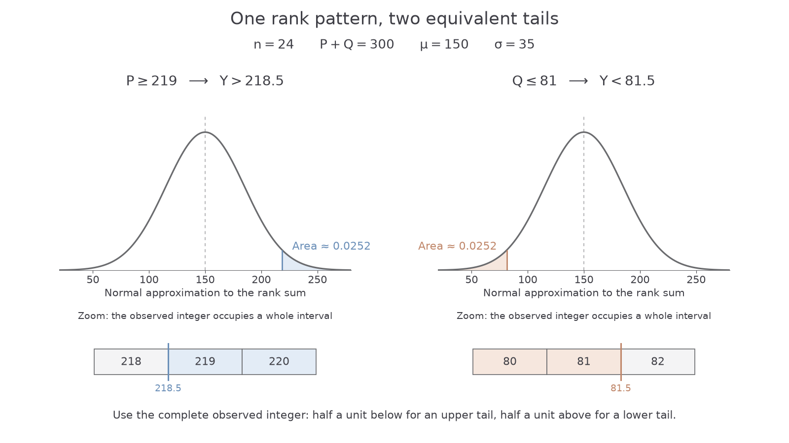
Change only the alternative. Here the two-sided result is close enough to the boundary that retaining intermediate precision matters.
Worked example 2: doubling a near-boundary tail
Question. For the same observations and , test against , at , using a normal approximation.
Plan. Use the same corrected tail and include its equally extreme reflected tail.
The null model is still , and the corrected upper-tail standardised value is still . Therefore
Do not round the standardised value to before making this comparison.
Answer. Do not reject using this normal approximation. There is insufficient evidence at the level that the population median differs from .
Check. The two-sided normal cutoff is approximately , slightly larger than . The critical-value comparison gives the same decision.
The table and the approximation concern the same null sign allocations. Use the supplied exact table when it covers the sample size; the large-sample calculation has approximation error, especially when its result lies near a decision boundary.
Watch out
The smaller sum is folded towards the lower end and is not normally distributed with the displayed mean. Choose or , then select its tail.
Use the lower positive-rank tail in this fresh test.
Large-sample rank-sum distribution
For two independent samples, the null distribution depends on both sample sizes, rather than on the number of paired differences.
Pool the observations and rank them increasingly. Let the smaller sample have size , with sum . Under the identical-populations null, each pooled rank has the same chance of belonging to this sample. Its mean rank is , so the expected sum is .
The ranks assigned to one sample are selected without replacement and are dependent. Do not calculate their variance as if they were independent uniform draws; use the supplied rank-sum variance.
Large-sample rank-sum model
For sufficiently large independent samples satisfying the rank-sum assumptions, under of identical populations,
Both formulae are in the formula booklet. This model approximates , not .
The populations must still be continuous and symmetric about their medians, with independent random samples and no pooled ties. Use the actual , and a half-unit continuity correction for the integer rank sum.
Continue this lesson.
You’re previewing NovaLearn without an account. Create a free account to read the rest.
Create free account