4.2 - The one-sample t-test

Normal samples with unknown variance

Sixteen measurements have mean $12.6$ and estimated standard deviation $1.2$. Is that convincing evidence that the population mean exceeds $12$? The difference $0.6$ matters only in relation to the uncertainty in the sample mean.

For a small random sample, the one-sample t procedure assumes independent observations from a normal population. The population variance $\sigma^2$ is unknown: we estimate it from the sample. A small sample does not make a non-normal population normal. Random sampling and the model assumptions are separate requirements.

Recall why the divisor in an unbiased variance estimate is one less than the sample size. The deviations from the fitted sample mean sum to zero: once $n-1$ deviations are known, the last is fixed. Estimating the mean has used one degree of freedom.

Unbiased means that over repeated samples the estimate averages to the true population variance; an individual estimate can be above or below it. The booklet also gives the descriptive standard deviation with divisor $n$. That describes the observed data; it is not the unbiased variance estimate used in this t-test.

Now change only the way the same information is supplied. Summarised data need the same correction for estimating the mean.

Keep the variance and standard deviation distinct: the t statistic below divides by a standard error, not by a variance.

The t statistic

The t statistic measures how far the sample mean is from the claimed population mean in estimated standard-error units.

If the population standard deviation were known, standardising a normal sample mean would give a standard normal variable. Replacing that fixed standard deviation by the random estimate $S$ adds uncertainty. The resulting t-distribution is symmetric about zero, with heavier tails than the standard normal distribution; its shape depends on the degrees of freedom.

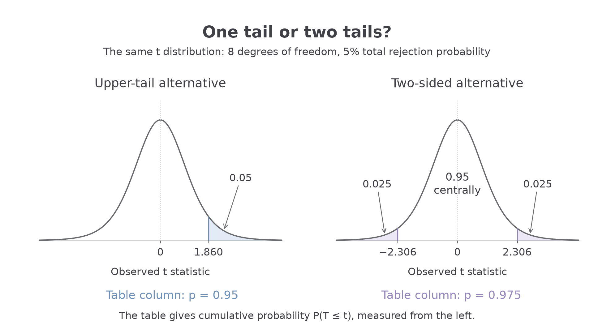
The table gives $t_{\nu,p}$ satisfying $P(T\le t_{\nu,p})=p$, not an upper-tail probability of $p$. At significance level $\alpha$, an upper-tail test uses $p=1-\alpha$; a two-tail test puts $\alpha/2$ in each tail and uses $p=1-\alpha/2$. For a lower-tail test, use symmetry to negate the corresponding positive value.

[DIAGRAM: asset_name: One tail or two tails; asset_slug: cam9231-t-test-tails; caption: At 5% significance, one upper tail starts at 1.860 but two tails start at plus or minus 2.306 for eight degrees of freedom; description: Two exact t density plots with eight degrees of freedom. The left plot shades the upper 0.05 tail beyond 1.860. The right plot shades two 0.025 tails beyond minus 2.306 and 2.306. The unshaded central probability is labelled 0.95 on the right. Labels distinguish the cumulative table columns p equals 0.95 and p equals 0.975.]