3.2.3.4 - Macroeconomic policy conflicts

Output gaps and policy conflicts

The state of demand relative to sustainable capacity helps explain whether a policy mainly improves output and employment or adds inflationary pressure.

With a negative output gap, actual real GDP is below potential and cyclical unemployment is present. Stronger AD can increase sales, output and derived demand for labour, so unemployment falls as unused capacity is brought into production. When SRAS is relatively responsive, much of the demand increase raises real output; price pressure may be limited. Near or above sustainable potential, bottlenecks, overtime and competition for workers make further AD expansion more likely to raise costs and prices. A positive output gap is associated with inflationary pressure; restraining demand can ease that pressure but may reduce employment and growth in the short run.

Use the same output-gap method as in the growth lesson: $(\text{actual}-\text{potential})/\text{potential}\times100$. In an illustrative economy with actual output 480 and potential 500, the gap is −4%. At actual 510 with unchanged potential, it is +2%. A gap is an estimated level comparison, not the GDP growth rate or an unemployment-rate calculation.

AD/AS reveals a key limitation of a simple inflation–unemployment trade-off. A leftward SRAS shift can raise prices and lower output simultaneously, increasing unemployment. Raising interest rates to restrain demand after such a shock may reduce second-round inflation pressure while worsening the output loss. Keeping demand high may protect activity temporarily while allowing more price pressure. The size and persistence of the shock and inflation expectations determine the severity of this conflict.

For example, the Bank of England's November 2022 report described higher gas prices and weaker household purchasing power alongside inflation pressures. This dated cost-shock context explains why the choice could not be understood as demand management moving along a single stable curve. A supply shock, demand changes and expectations can operate together.

The short-run Phillips curve

The short-run Phillips curve (SRPC) shows a possible inverse relationship between inflation and unemployment, holding expected inflation and supply conditions constant.

When AD strengthens, firms expand production and hire more workers. Tighter labour and product markets can increase wage and price pressure: unemployment falls while inflation rises. Demand restraint can reverse this movement. The curve describes a conditional short-run relationship, rather than a menu policymakers can choose from forever.

The illustrative diagram below uses $\pi=\pi^e-2(u-5)$, where $\pi$ is annual inflation in percent, $\pi^e$ is expected inflation and $u$ is unemployment in percent. With expected inflation 2%, the blue SRPC contains A at (5%,2%) and B at (4%,4%). A demand expansion can move A→B while expectations remain fixed. These chosen numbers teach the model and are not an estimated UK trade-off.

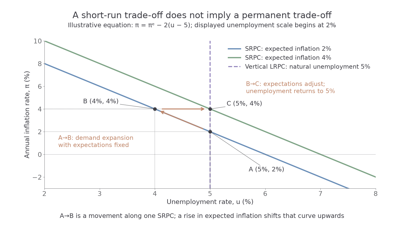
In a notebook, label unemployment rate horizontally and inflation rate, rather than price level, vertically. Draw the downward SRPC, name the expected inflation underlying it and identify a movement between points. A change in expected inflation or a supply shock shifts the SRPC; it is not a movement along the old one. A supply shock can worsen inflation and unemployment together, so an observed correlation does not prove demand caused the change.

The long-run Phillips curve and expectations

The vertical long-run Phillips curve (LRPC) shows unemployment returning to its natural rate when expectations and wages have adjusted; permanently higher inflation does not permanently buy lower unemployment in this model.

AQA also calls this the “L-shaped” long-run Phillips curve, and identifies it as the vertical long-run curve. The required long-run implication is verticality at the natural rate, not a permanently downward inflation–unemployment trade-off. In the supplied diagram, the illustrative natural rate is 5%, so the LRPC is the vertical line at 5% unemployment. Natural unemployment includes normal search and mismatch; it is not zero or immutable.