3.1.5.3 - Perfect competition

Why the firm takes the price

In perfect competition, many small producers supply an identical product, buyers and sellers have perfect relevant knowledge, and firms can enter and leave freely. Each firm is too small to change total market supply appreciably. Buyers can obtain the same product from others, so a firm charging above the market price loses its customers. Charging less is unnecessary when it can sell its feasible output at the going price.

The industry's demand curve slopes downward, but the individual firm's demand is horizontal at the market price. Do not confuse these two graphs. For the firm, price equals average revenue and marginal revenue: $P=AR=MR$. It chooses how much to produce, not a separate market price. The profit-maximising condition is MC=MR on the rising relevant MC curve, so its chosen output satisfies P=MC.

Perfect knowledge helps customers compare identical offers and lets firms recognise profitable opportunities. Free entry prevents sustained economic profits in the long-run benchmark; free exit lets loss-making resources move elsewhere. These assumptions do different jobs. A market can have many firms yet fail the benchmark because products differ, consumers cannot compare prices or entry is blocked.

Short-run profit and loss

In the short run, some productive inputs are fixed and the number of firms cannot fully adjust. A firm can earn economic profit, normal profit or a loss, depending on price relative to average cost at its chosen output.

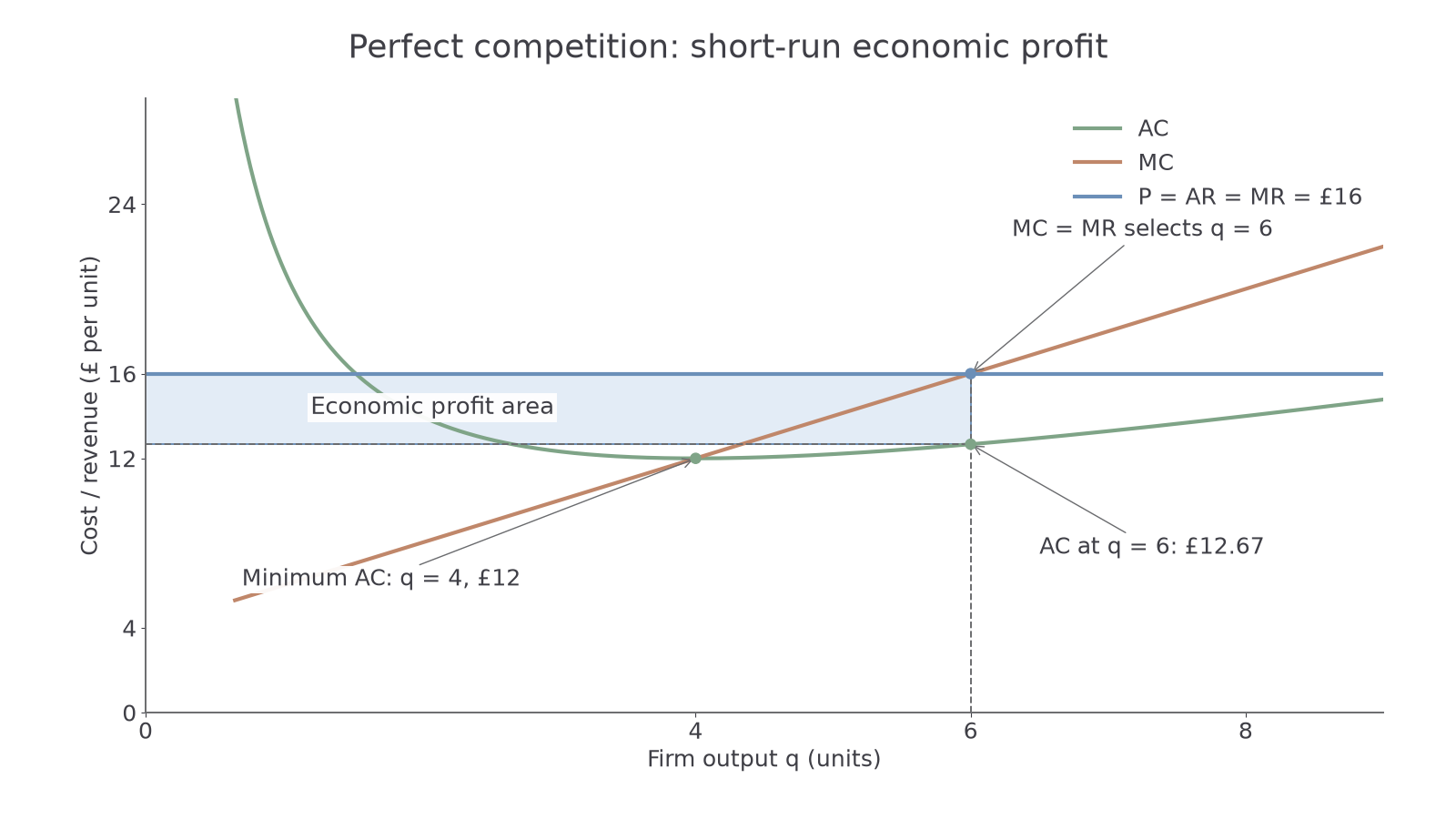
In this original cost model, $TC=16+4q+q^2$, $AC=16/q+4+q$ and $MC=4+2q$. The graph's horizontal price line is £16, so MC=MR selects 6 units. AC there is £12.67 approximately, not the minimum AC. Total revenue is £96 and total cost is £76: economic profit is £20. The shaded rectangle's exact height is $16-76/6$ and width 6, giving £20. Normal profit is already included in AC; economic profit is the surplus above it.

For a notebook diagram, label output horizontally and cost/revenue per unit vertically. Draw AC and MC so MC crosses AC at its minimum. Add horizontal P=AR=MR, choose the rising MC intersection, and project that output to AC. Shade the rectangle between P and AC only over the chosen output. Do not select output at minimum AC unless it also satisfies MC=MR.

If P is below AC, the chosen output makes a loss. That does not always mean immediate closure. A firm continues in the short run if revenue covers variable costs and contributes toward fixed costs; P above average variable cost (AVC) permits this. In the model, at P=10, q=3, AVC=7 and AC≈12.33. Operating loses £7, less than the £16 fixed-cost loss from closing. Below minimum AVC, production cannot cover variable costs, so shutdown is preferable. At the threshold the firm is indifferent. This compares avoidable costs; sunk fixed costs should not determine the extra-unit decision.

Entry, exit and long-run equilibrium

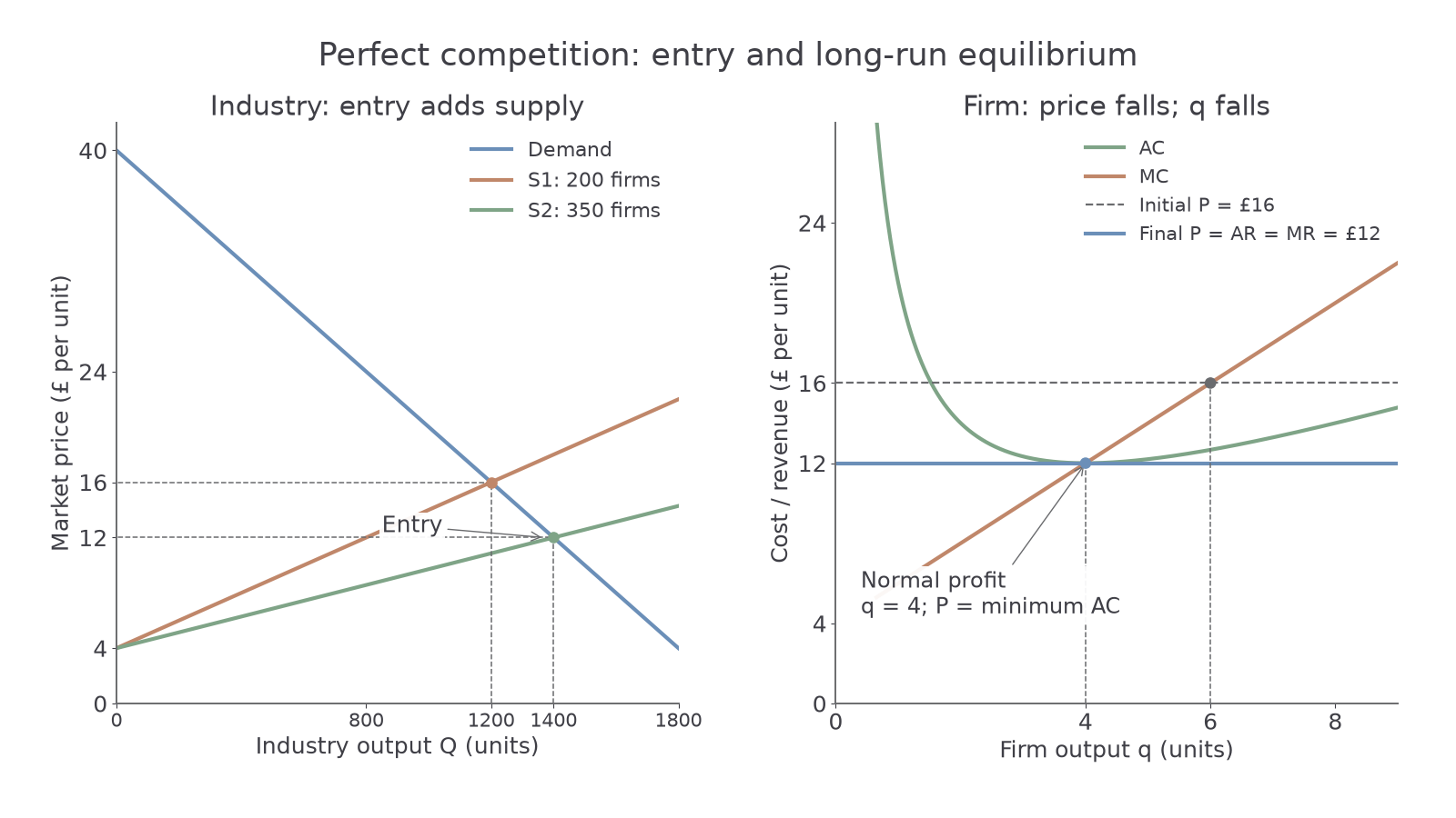
Economic profits attract entry when no barriers prevent it. Additional firms shift industry supply right, reducing the market price. Each existing firm's horizontal demand line moves down, and it moves to a lower output on its MC curve. Entry stops in the standard identical-firm, constant-cost model when only normal profit remains. Losses induce exit, shifting industry supply left and raising price until remaining firms cover their full economic costs.