3.1.4.6 - Revenue and revenue curves
Learn to calculate total, average and marginal revenue, and explain why they behave differently when a firm changes its sales. Connect numerical tables to revenue curves and use them to judge the revenue effect of a price change.
Total, average and marginal revenue
Revenue is the income a firm receives from selling output before deducting its production costs. A high revenue figure alone therefore does not establish a high profit.
Revenue measures
Total revenue (TR) is the revenue from all units sold. Average revenue (AR) is revenue per unit. Marginal revenue (MR) is the extra total revenue from an additional unit; when data show a larger output interval, the formula gives extra revenue per unit over that interval. Use the change in quantity, not the final quantity, as the MR denominator.
In this original illustrative table, a seller charges one common price for all units sold at each output:
| Quantity sold per day | Price per unit | Total revenue per day | Average revenue | MR of the additional unit |
|---|---|---|---|---|
| 0 | — | £0 | — | — |
| 1 | £11 | £11 | £11 | £11 |
| 2 | £10 | £20 | £10 | £9 |
| 3 | £9 | £27 | £9 | £7 |
| 4 | £8 | £32 | £8 | £5 |
At four units, and . Revenue rises from £27 to £32 when the fourth unit is sold, so its MR is £5, not its £8 selling price. AR is undefined at zero output because division by zero is undefined; TR can still be zero.
For a larger interval, if TR rises from £200 to £272 when output rises from 20 to 24 units, per extra unit on average over the interval. The data do not establish the MR of each individual unit separately.
Demand, average revenue and marginal revenue
The firm's demand curve is its AR curve when every unit at a given output is sold at the same price. Demand shows the price customers will pay for that quantity, and . Thus the vertical coordinate represents both price and average revenue.
With downward-sloping demand, selling more usually requires a lower price. MR lies below AR because the extra sale brings in revenue while the price cut reduces revenue on units that could have been sold at the old price. This applies to a firm charging a common price, rather than charging each customer a different price.
For example, an illustrative seller can sell five subscriptions at £10 each or six at £9 each. The sixth sale contributes £9, but the £1 price cut reduces revenue on the original five subscriptions by £5. MR is consequently £4: total revenue rises from £50 to £54. The sixth customer's payment is not the whole revenue change.
For straight-line demand, the continuous MR curve has the same vertical intercept as AR and twice its downward slope. It reaches the output axis halfway to AR's output intercept. These are properties of linear demand, not rules for every possible curved demand function.
A movement along AR represents the firm choosing a different price and quantity under unchanged demand conditions. Increased customer income or popularity may shift demand and therefore AR; the associated MR curve changes too. An increase in production cost does not by itself shift the revenue curves: it changes costs, although the firm may respond by choosing a different output.
Revenue at a constant market price
A price-taking firm can sell the relevant range of output at an unchanged market price. Each additional unit earns the same amount, so price, AR and MR are equal.
If the illustrative market price is £8, two units produce TR of £16 and five produce TR of £40. Each extra unit adds £8. AR and MR are horizontal lines at £8; TR is a straight line through the origin whose slope is £8 per unit.
This is a model of the firm's demand, not necessarily the entire market's demand. The market price is determined by aggregate demand and supply. An individual small firm takes it as given because its own output change has a negligible effect on that price. The firm's horizontal demand assumption does not mean every producer could expand simultaneously without affecting the market price.
To draw these curves in a notebook, use quantity on each horizontal axis. Put pounds per unit on the AR/MR panel and pounds of total revenue on a separate TR panel. Draw the shared AR = MR line at the given price and the rising TR line from zero. A change in the market price shifts the horizontal line and changes TR's slope; merely selling more at the same price is a movement along the existing curves.
Linking marginal and total revenue
Marginal revenue shows how total revenue changes as output increases. Positive MR means TR is rising; zero MR marks a stationary TR point; negative MR means TR is falling. In the usual single-peaked revenue model, TR is at its maximum where MR changes from positive to negative through zero.
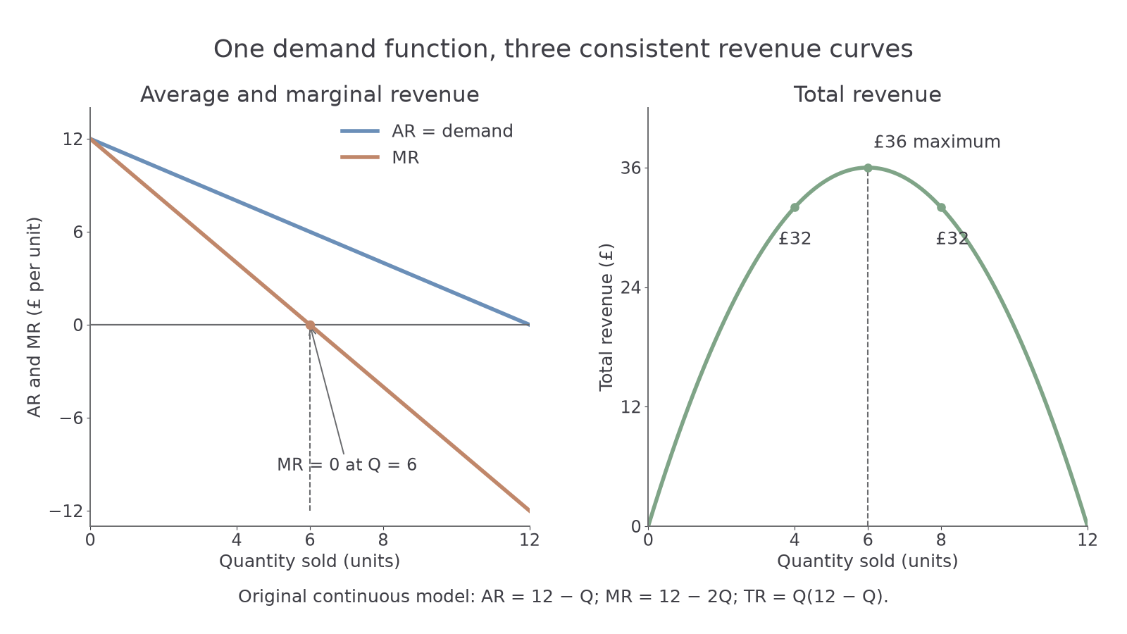
The original illustrative graph uses , so . Its continuous MR is . At , AR is £8, MR is £4 and TR is £32. At , AR is £6 and MR is zero, while TR reaches £36. Expanding to reduces TR to £32, and point MR is −£4. Negative MR means the price reduction on existing sales outweighs revenue from extra sales; it does not mean customers pay a negative price.
The continuous MR curve describes the slope of TR at a point. A discrete table instead gives changes over intervals. For the same function, TR rises from £35 at five units to £36 at six, so MR of that one-unit interval is £1; the curve's MR at exactly six units is zero. There is no contradiction: one measures the average change over the interval and the other the slope at its endpoint. Do not attach an interval MR to a point on the continuous curve without explaining the convention.
To construct the supplied graph in a notebook, mark AR at £12 when and zero when . Draw MR from the same £12 intercept to zero at , continuing below the axis. In a separate panel, plot TR at zero, 4, 6, 8 and 12 units as £0, £32, £36, £32 and £0. Use a smooth curve joining these points. The highest TR point aligns vertically with MR = 0. Keep the total and per-unit scales distinct.
Price changes and revenue decisions
Price elasticity helps explain whether extra sales compensate for a lower price. Where demand is price elastic, a price cut creates a proportionately larger quantity increase and TR rises. Where demand is price inelastic, the quantity response is proportionately smaller and TR falls. The corresponding MR is positive in the elastic region and negative in the inelastic region; on a smooth demand curve, unit elasticity occurs at the TR maximum.
In the graph, reducing price from £8 to £6 raises quantity from four to six and TR from £32 to £36. A further reduction from £6 to £4 increases quantity from six to eight but reduces TR to £32. The same direction of price change therefore has a different revenue effect in different demand regions. Elasticity is not constant merely because demand is a straight line.
For a separate illustrative example, a price reduction from £10 to £8 that raises sales from 100 to 150 units increases TR from £1,000 to £1,200. The increase in sales more than compensates for the price reduction. If sales rose only to 110, TR would instead be £880. Calculate both price-times-quantity totals before making a claim from “sales increased”.
The firm must also consider costs. Maximising revenue is not necessarily maximising profit, since extra output uses resources. If the next units add more to cost than to revenue, producing them can reduce profit even while TR is rising. Use MR to describe the revenue effect; a profit decision requires cost information as well.
Quick Recap
TR measures all sales income, AR measures revenue per unit and MR measures the change in TR per extra unit. Common-price demand is AR; downward-sloping demand puts MR below AR. MR links the direction of TR change to elasticity, while cost information is needed to infer profit.