3.1.5.11 - Consumer and producer surplus

Surplus from exchange

Consumer and producer surplus measure gains from exchange relative to willingness to pay and the variable opportunity cost of supply.

Consumer surplus is the difference between what buyers are willing to pay and what they actually pay. On a demand diagram it is the area below demand and above the price, up to the quantity purchased. Producer surplus is revenue above variable opportunity cost: the area above the supply curve or MC curve and below the price, over the units supplied. With fixed economic costs, producer surplus is not economic profit; deduct those fixed costs to obtain profit.

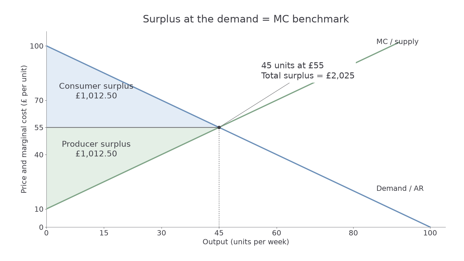
This original illustrative industry has demand $P=100-Q$ and supply/MC $P=10+Q$. Output is units per week and price/cost is pounds per unit. Their intersection is 45 units at £55. Demand's vertical intercept is £100; MC's is £10. For straight lines, use:

Consumer surplus is $\tfrac12\times45\times(100-55)=£1,012.50$ per week. Producer surplus is $\tfrac12\times45\times(55-10)=£1,012.50$ per week. Total surplus is £2,025. The areas have monetary units: pounds per unit multiplied by units per week gives pounds per week.

To construct the diagram in a notebook, label axes and units, draw demand and MC/supply, identify their intersection, and draw the horizontal transaction price. Shade consumer surplus above price but below demand, and producer surplus below price but above MC, stopping both at traded output. A curved boundary needs its actual area; do not apply the triangle formula to every demand or supply shape.

These measures reflect willingness and ability to pay, not equal welfare weights for rich and poor. The sum is a useful efficiency measure when demand represents marginal social benefit and MC marginal social cost, with no unpriced externalities. Fixed costs common to the alternatives can be subtracted from both totals without changing their difference. A distributional judgement or a market with external costs requires more than these private surplus areas.

Monopoly welfare loss

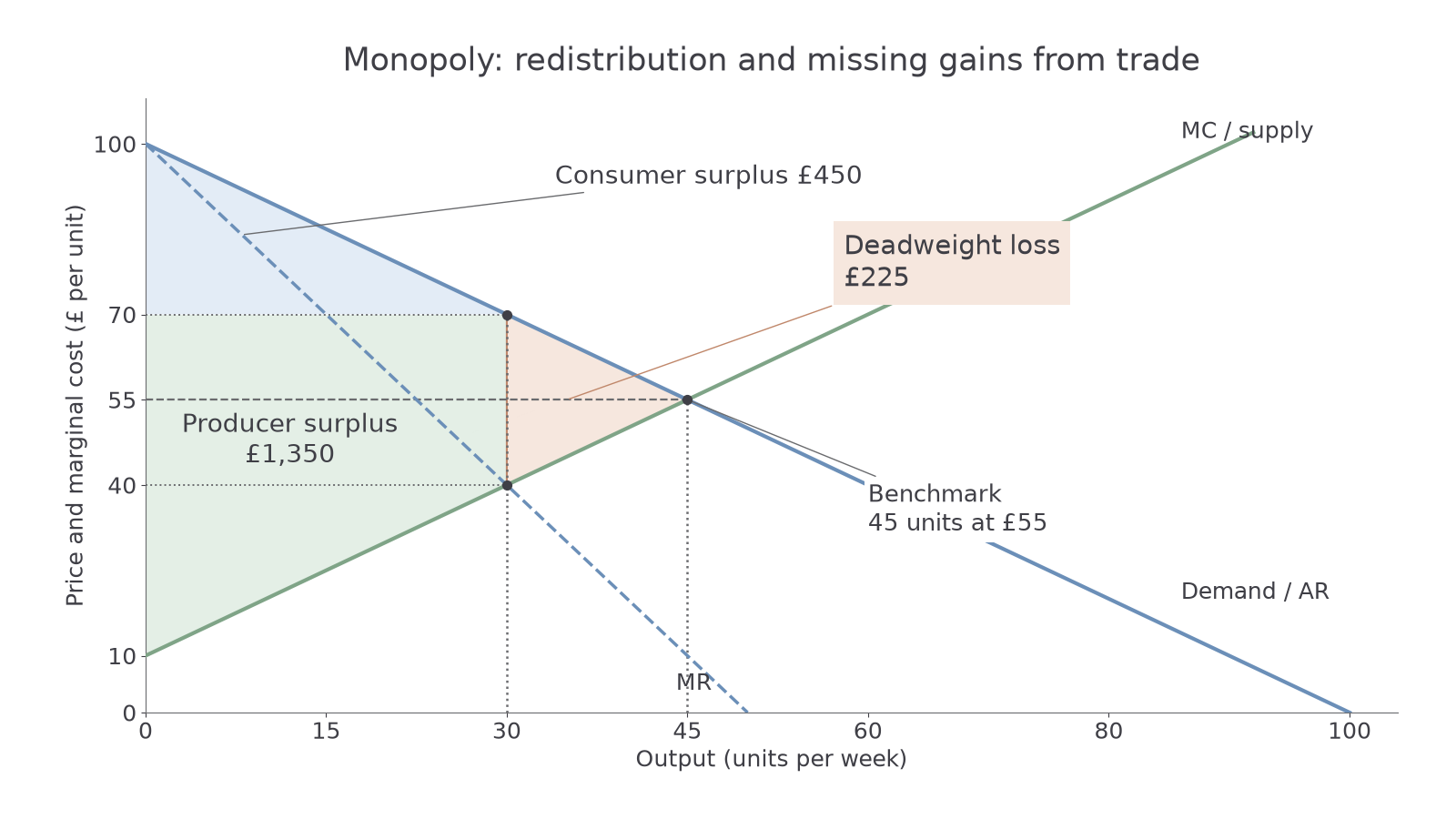
A single-price monopoly can transfer surplus to the producer and eliminate gains from trades that no longer occur.

Use the same illustrative demand and MC as in the competitive benchmark, holding technology and preferences constant. A single-price profit-maximising monopolist has MR $=100-2Q$. MR = MC gives 30 units, and demand gives price £70. The benchmark where demand = MC remains 45 units at £55.