3.2.2.2 - Aggregate demand and aggregate supply

Price level and real output

An AD/AS diagram describes the whole economy, with price level on the vertical axis and real national output on the horizontal axis. It is not the price and quantity of one product. A price index such as 100 or 110 is a level; inflation is the rate at which that level changes over time.

Aggregate demand (AD) is planned spending on domestic goods and services at each price level. It is commonly written $AD=C+I+G+(X-M)$. Holding other determinants constant, a lower price level can increase real wealth and spending, reduce the demand for money and borrowing costs, and improve domestic price competitiveness relative to overseas output. These channels help explain a downward-sloping AD curve. Their strength depends on financial conditions, exchange rates and the response of spending; the individual-market substitution story alone is insufficient.

Short-run aggregate supply (SRAS) is the real output firms are willing to supply at each price level while some input prices and contracts are slow to adjust. Higher selling prices relative to sticky costs make additional production more profitable, giving an upward slope. A change in the price level alone is a movement along an existing AD or SRAS curve. A change in another determinant alters desired spending or production at every price level, shifting the relevant curve.

Finding macroeconomic equilibrium

At the intersection of AD and SRAS, planned real expenditure equals output supplied at the prevailing price level. Label it $E_0$, then project horizontally to $P_0$ and vertically to $Y_0$. Above that price level, desired supply exceeds demand in the simple model; unsold output puts downward pressure on prices and production. Below it, excess demand puts upward pressure on prices and production. This is a model of adjustment, not a claim that all prices change instantly.

To construct a diagram in a notebook: label both axes and the curves, locate the initial intersection, draw and label the shifted curve only after identifying the changed determinant, locate its new intersection with the unchanged curve, and compare both axis coordinates. Keep the direction of the shift separate from any movement along the unchanged curve. Use a symbolic scale unless actual data are supplied.

The two panels below are exact illustrative models, not estimates of a real economy. Each begins at $Y_0=100$, $P_0=100$, with annual real output in billions of base-year pounds. The demand shock leads to $(80,90)$; the cost shock leads to $(80,110)$.

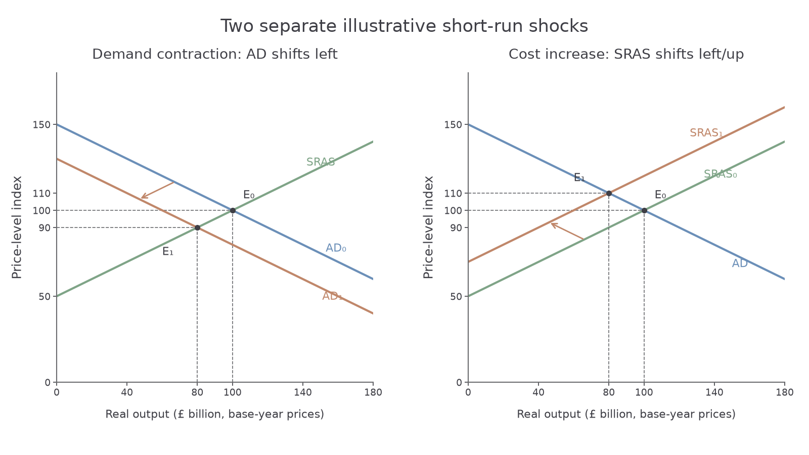
In the left panel, AD shifts left while SRAS stays fixed, so the economy moves down SRAS. In the right panel, SRAS shifts left/up while AD stays fixed, so the economy moves up AD. Neither unchanged curve should also shift merely because the new equilibrium has a different price level.

Demand shocks and unemployment

A demand-side shock changes a component of spending at a given price level. Reduced consumer confidence can lead households to postpone purchases; higher borrowing costs can deter consumption and investment; lower overseas income can reduce exports. Each can shift AD left. Extra government purchases or a recovery in foreign demand can shift it right, holding other factors constant.

With upward-sloping SRAS, lower AD reduces real output and the price level. Firms need fewer labour hours to meet lower sales, so unemployment may rise. If output is below normal capacity because demand is weak, the additional unemployment is demand-deficient, or cyclical. The output fall alone does not prove all unemployment is cyclical: skill mismatches and other supply-side causes can coexist.